ode23t
Solve moderately stiff ODEs and DAEs — trapezoidal rule
Syntax
Description
[, wheret,y] = ode23t(odefun,tspan,y0)tspan = [t0 tf], integrates the system of differential equations
fromt0totfwith initial conditionsy0。Each row in the solution arrayycorresponds to a value returned in column vectort。
All MATLAB®ODE solvers can solve systems of equations of the form
, or problems that involve a mass matrix,
。解决所有使用类似的语法。的ode23ssolver only can solve problems with a mass matrix if the mass matrix is constant.ode15sandode23tcan solve problems with a mass matrix that is singular, known as differential-algebraic equations (DAEs). Specify the mass matrix using theMassoption ofodeset。
[additionally finds where functions of(t,y), called event functions, are zero. In the output,t,y,te,ye,ie] = ode23t(odefun,tspan,y0,options)teis the time of the event,yeis the solution at the time of the event, andieis the index of the triggered event.
For each event function, specify whether the integration is to terminate at a zero and whether the direction of the zero crossing matters. Do this by setting the'Events'property to a function, such asmyEventFcnor@myEventFcn, and creating a corresponding function: [value,isterminal,direction] =myEventFcn(t,y). For more information, seeODE Event Location。
sol= ode23t(___)devalto evaluate the solution at any point on the interval[t0 tf]。You can use any of the input argument combinations in previous syntaxes.
Examples
ODE With Single Solution Component
Simple ODEs that have a single solution component can be specified as an anonymous function in the call to the solver. The anonymous function must accept two inputs(t,y), even if one of the inputs is not used in the function.
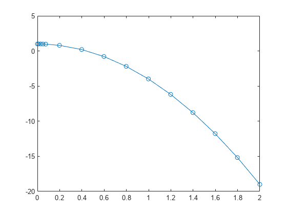
Solve the ODE
Specify a time interval of[0 2]and the initial conditiony0 = 1。
tspan = [0 2]; y0 = 1; [t,y] = ode23t(@(t,y) -10*t, tspan, y0);
Plot the solution.
plot(t,y,'-o')
Solve Stiff ODE
An example of a stiff system of equations is the van der Pol equations in relaxation oscillation. The limit cycle has regions where the solution components change slowly and the problem is quite stiff, alternating with regions of very sharp change where it is not stiff.
的system of equations is:

的initial conditions are and
and 。的function
vdp1000ships with MATLAB® and encodes the equations.
functiondydt = vdp1000(t,y)%VDP1000 Evaluate the van der Pol ODEs for mu = 1000.%% See also ODE15S, ODE23S, ODE23T, ODE23TB.% Jacek Kierzenka and Lawrence F. Shampine% Copyright 1984-2014 The MathWorks, Inc.dydt = [y(2); 1000*(1-y(1)^2)*y(2)-y(1)];
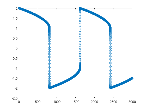
Solving this system usingode45with the default relative and absolute error tolerances (1e-3and1e-6, respectively) is extremely slow, requiring several minutes to solve and plot the solution.ode45requires millions of time steps to complete the integration, due to the areas of stiffness where it struggles to meet the tolerances.
This is a plot of the solution obtained byode45, which takes a long time to compute. Notice the enormous number of time steps required to pass through areas of stiffness.
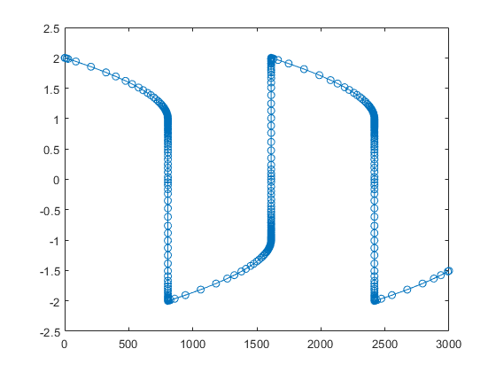
Solve the stiff system using theode23tsolver, and then plot the first column of the solutionyagainst the time pointst。的ode23tsolver passes through stiff areas with far fewer steps thanode45。
[t,y] = ode23t(@vdp1000,[0 3000],[2 0]); plot(t,y(:,1),'-o')
Pass Extra Parameters to ODE Function
ode23tonly works with functions that use two input arguments,tandy。不过,您可以通过在def额外参数ining them outside the function and passing them in when you specify the function handle.
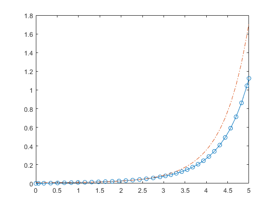
Solve the ODE

Rewriting the equation as a first-order system yields

odefcn.mrepresents this system of equations as a function that accepts four input arguments:t,y,A, andB。
functiondydt = odefcn(t,y,A,B) dydt = zeros(2,1); dydt(1) = y(2); dydt(2) = (A/B)*t.*y(1);
Solve the ODE usingode23t。Specify the function handle such that it passes in the predefined values forAandBtoodefcn。
A = 1; B = 2; tspan = [0 5]; y0 = [0 0.01]; [t,y] = ode23t(@(t,y) odefcn(t,y,A,B), tspan, y0);
Plot the results.
plot(t,y(:,1),'-o',t,y(:,2),'-.')
Compare Stiff ODE Solvers
的ode15ssolver is a good first choice for most stiff problems. However, the other stiff solvers might be more efficient for certain types of problems. This example solves a stiff test equation using all four stiff ODE solvers.
Consider the test equation
的equation becomes increasingly stiff as the magnitude of
increases. Use
and the initial condition
over the time interval[0 0.5]。With these values, the problem is stiff enough thatode45andode23struggle to integrate the equation. Also, useodesetto pass in the constant Jacobian
and turn on the display of solver statistics.
lambda = 1e9; y0 = 1; tspan = [0 0.5]; opts = odeset('Jacobian',-lambda,'Stats','on');
Solve the equation withode15s,ode23s,ode23t, andode23tb。Make subplots for comparison.
subplot(2,2,1) tic, ode15s(@(t,y) -lambda*y, tspan, y0, opts), toc
104 successful steps 1 failed attempts 212 function evaluations 0 partial derivatives 21 LU decompositions 210 solutions of linear systems Elapsed time is 1.505900 seconds.
title('ode15s') subplot(2,2,2) tic, ode23s(@(t,y) -lambda*y, tspan, y0, opts), toc
63 successful steps 0 failed attempts 191 function evaluations 0 partial derivatives 63 LU decompositions 189 solutions of linear systems Elapsed time is 0.439813 seconds.
title('ode23s') subplot(2,2,3) tic, ode23t(@(t,y) -lambda*y, tspan, y0, opts), toc
95 successful steps 0 failed attempts 125 function evaluations 0 partial derivatives 28 LU decompositions 123 solutions of linear systems Elapsed time is 0.598499 seconds.
title('ode23t') subplot(2,2,4) tic, ode23tb(@(t,y) -lambda*y, tspan, y0, opts), toc
71 successful steps 0 failed attempts 167 function evaluations 0 partial derivatives 23 LU decompositions 236 solutions of linear systems Elapsed time is 0.600518 seconds.
title('ode23tb')
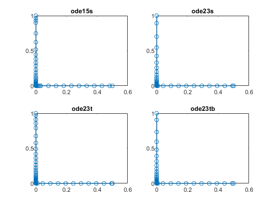
的stiff solvers all perform well, butode23scompletes the integration with the fewest steps and runs the fastest for this particular problem. Since the constant Jacobian is specified, none of the solvers need to calculate partial derivatives to compute the solution. Specifying the Jacobian benefitsode23sthe most since it normally evaluates the Jacobian in every step.
For general stiff problems, the performance of the stiff solvers varies depending on the format of the problem and specified options. Providing the Jacobian matrix or sparsity pattern always improves solver efficiency for stiff problems. But since the stiff solvers use the Jacobian differently, the improvement can vary significantly. Practically speaking, if a system of equations is very large or needs to be solved many times, then it is worthwhile to investigate the performance of the different solvers to minimize execution time.
Input Arguments
Output Arguments
Algorithms
ode23tis an implementation of the trapezoidal rule using a “free” interpolant. This solver is preferred overode15sif the problem is only moderately stiff and you need a solution without numerical damping.ode23talso can solve differential algebraic equations (DAEs)[1],[2]。
References
[1] Shampine, L. F., M. W. Reichelt, and J.A. Kierzenka, “Solving Index-1 DAEs in MATLAB and Simulink”,SIAM Review, Vol. 41, 1999, pp. 538–552.
[2] Shampine, L. F. and M. E. Hosea, “Analysis and Implementation of TR-BDF2,”Applied Numerical Mathematics 20, 1996.
See Also
选择a Web Site
Choose a web site to get translated content where available and see local events and offers. Based on your location, we recommend that you select:。
选择web siteYou can also select a web site from the following list:
Americas
- América Latina(Español)
- Canada(English)
- United States(English)
Europe
- Belgium(English)
- Denmark(English)
- Deutschland(Deutsch)
- España(Español)
- Finland(English)
- France(Français)
- Ireland(English)
- Italia(Italiano)
- Luxembourg(English)
- Netherlands(English)
- Norway(English)
- Österreich(Deutsch)
- Portugal(English)
- Sweden(English)
- Switzerland
- United Kingdom(English)