portsim
Monte Carlo simulation of correlated asset returns
Syntax
Description
RetSeries= portsim(ExpReturn,ExpCovariance,NumObs)NASSETSassets overNUMOBSconsecutive observation intervals. Asset returns are simulated as the proportional increments of constant drift, constant volatility stochastic processes, thereby approximating continuous-time geometric Brownian motion.
Note
An alternative for portfolio optimization is to use thePortfolioobject for mean-variance portfolio optimization. This object supports gross or net portfolio returns as the return proxy, the variance of portfolio returns as the risk proxy, and a portfolio set that is any combination of the specified constraints to form a portfolio set. For information on the workflow when usingPortfolioobjects, seePortfolio Object Workflow.
RetSeries= portsim(___,RetIntervals,NumSim,Method)
Examples
Distinction Between Simulation Methods
This example shows the distinction between theExactandExpectedmethods of simulation.
Consider a portfolio of five assets with the following expected returns, standard deviations, and correlation matrix based on daily asset returns (whereExpReturnandSigmasare divided by 100 to convert percentages to returns).
ExpReturn = [0.0246 0.0189 0.0273 0.0141 0.0311]/100; Sigmas = [0.9509 1.4259 1.5227 1.1062 1.0877]/100; Correlations = [1.0000 0.4403 0.4735 0.4334 0.6855 0.4403 1.0000 0.7597 0.7809 0.4343 0.4735 0.7597 1.0000 0.6978 0.4926 0.4334 0.7809 0.6978 1.0000 0.4289 0.6855 0.4343 0.4926 0.4289 1.0000];
Convert the correlations and standard deviations to a covariance matrix.
ExpCovariance = corr2cov(Sigmas, Correlations)
ExpCovariance =5×510-3× 0.0904 0.0597 0.0686 0.0456 0.0709 0.0597 0.2033 0.1649 0.1232 0.0674 0.0686 0.1649 0.2319 0.1175 0.0816 0.0456 0.1232 0.1175 0.1224 0.0516 0.0709 0.0674 0.0816 0.0516 0.1183
Assume that there are 252 trading days in a calendar year, and simulate two sample paths (realizations) of daily returns over a two-year period. SinceExpReturnandExpCovarianceare expressed daily, setRetIntervals = 1.
StartPrice = 100; NumObs = 504;% two calendar years of daily returnsNumSim = 2; RetIntervals = 1;% one trading dayNumAssets = 5;
To illustrate the distinction between methods, simulate two paths by each method, starting with the same random number state.
rng('default'); RetExact = portsim(ExpReturn, ExpCovariance, NumObs,...RetIntervals, NumSim,'Exact'); rng(0); RetExpected = portsim(ExpReturn, ExpCovariance, NumObs,...RetIntervals, NumSim,'Expected');
Compare the mean and covariance ofRetExactwith the inputs (ExpReturnandExpCovariance), you will observe that they are almost identical.
At this point,RetExactandRetExpectedare both 504-by-5-by-2 arrays. Now assume an equally weighted portfolio formed from the five assets and create arrays of portfolio returns in which each column represents the portfolio return of the corresponding sample path of the simulated returns of the five assets. The portfolio arraysPortRetExactandPortRetExpectedare 504-by-2 matrices.
Weights = ones(NumAssets, 1)/NumAssets; PortRetExact = zeros(NumObs, NumSim); PortRetExpected = zeros(NumObs, NumSim);fori = 1:NumSim PortRetExact(:,i) = RetExact(:,:,i) * Weights; PortRetExpected(:,i) = RetExpected(:,:,i) * Weights;end
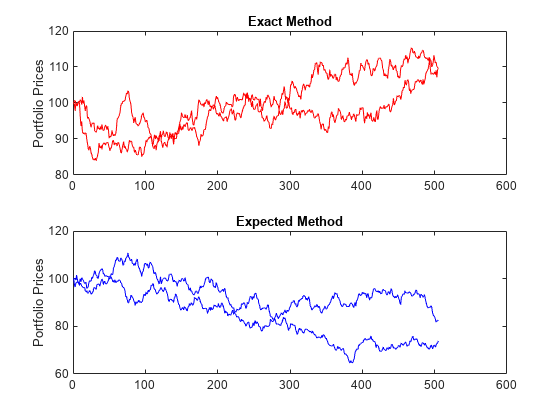
Finally, convert the simulated portfolio returns to prices and plot the data. In particular, note that since theExactmethod matches expected return and covariance, the terminal portfolio prices are virtually identical for each sample path. This is not true for theExpectedsimulation method. Although this example examines portfolios, the same methods apply to individual assets as well. Thus,Exactsimulation is most appropriate when unique paths are required to reach the same terminal prices.
PortExact = ret2tick(PortRetExact,...repmat(StartPrice,1,NumSim)); PortExpected = ret2tick(PortRetExpected,...repmat(StartPrice,1,NumSim)); subplot(2,1,1), plot(PortExact,'-r') ylabel('Portfolio Prices') title('Exact Method') subplot(2,1,2), plot(PortExpected,'-b') ylabel('Portfolio Prices') title('Expected Method')
Interaction BetweenExpReturn,ExpCovariance, andRetIntervals
This example shows the interplay amongExpReturn,ExpCovariance, andRetIntervals. Recall thatportsimsimulates correlated asset returns over an interval of lengthdt, given by the equation
whereSis the asset price,μis the expected rate of return,σ资产价格的波动,εrepresents a random drawing from a standardized normal distribution.
The time incrementdtis determined by the optional inputRetIntervals, either as an explicit input argument or as a unit time increment by default. Regardless, the periodicity ofExpReturn,ExpCovariance, andRetIntervalsmust be consistent. For example, ifExpReturnandExpCovarianceare annualized, thenRetIntervalsmust be in years. This point is often misunderstood.
To illustrate the interplay amongExpReturn,ExpCovariance, andRetIntervals, consider a portfolio of five assets with the following expected returns, standard deviations, and correlation matrix based on daily asset returns.
ExpReturn = [0.0246 0.0189 0.0273 0.0141 0.0311]/100; Sigmas = [0.9509 1.4259 1.5227 1.1062 1.0877]/100; Correlations = [1.0000 0.4403 0.4735 0.4334 0.6855 0.4403 1.0000 0.7597 0.7809 0.4343 0.4735 0.7597 1.0000 0.6978 0.4926 0.4334 0.7809 0.6978 1.0000 0.4289 0.6855 0.4343 0.4926 0.4289 1.0000];
Convert the correlations and standard deviations to a covariance matrix of daily returns.
ExpCovariance = corr2cov(Sigmas, Correlations);
Assume 252 trading days per calendar year, and simulate a single sample path of daily returns over a four-year period. Since theExpReturnandExpCovarianceinputs are expressed daily, setRetIntervals = 1.
StartPrice = 100; NumObs = 1008;% four calendar years of daily returnsRetIntervals = 1;% one trading dayNumAssets = length(ExpReturn); randn('state',0); RetSeries1 = portsim(ExpReturn, ExpCovariance, NumObs,...RetIntervals, 1,'Expected');
Now annualize the daily data, thereby changing the periodicity of the data, by multiplyingExpReturnandExpCovarianceby 252 and dividingRetIntervalsby 252 (RetIntervals= 1/252 of a year). Resetting the random number generator to its initial state, you can reproduce the results.
rng('default'); RetSeries2 = portsim(ExpReturn*252, ExpCovariance*252,...NumObs, RetIntervals/252, 1,'Expected');
Assume an equally weighted portfolio and compute portfolio returns associated with each simulated return series.
Weights = ones(NumAssets, 1)/NumAssets; PortRet1 = RetSeries2 * Weights; PortRet2 = RetSeries2 * Weights;
Comparison of the data reveals thatPortRet1andPortRet2are identical.
Univariate Geometric Brownian Motion
This example shows how to simulate a univariate geometric Brownian motion process. It is based on an example found in Hull,Options, Futures, and Other Derivatives, 5th Edition (see example 12.2 on page 236). In addition to verifying Hull's example, it also graphically illustrates the lognormal property of terminal stock prices by a rather large Monte Carlo simulation.
Assume that you own a stock with an initial price of $20, an annualized expected return of 20% and volatility of 40%. Simulate the daily price process for this stock over the course of one full calendar year (252 trading days).
StartPrice = 20; ExpReturn = 0.2; ExpCovariance = 0.4^2; NumObs = 252; NumSim = 10000; RetIntervals = 1/252;
RetIntervalsis expressed in years, consistent with the fact thatExpReturnandExpCovarianceare annualized. Also,ExpCovarianceis entered as a variance rather than the more familiar standard deviation (volatility).
Set the random number generator state, and simulate 10,000 trials (realizations) of stock returns over a full calendar year of 252 trading days.
rng('default'); RetSeries = squeeze(portsim(ExpReturn, ExpCovariance, NumObs,...RetIntervals, NumSim,'Expected'));
Thesqueezefunction reformats the output array of simulated returns from a252-by-1-by-10000array to more convenient252-by-10000array. (Recall thatportsimis fundamentally a multivariate simulation engine).
In accordance with Hull's equations 12.4 and 12.5 on page 236
convert the simulated return series to a price series and compute the sample mean and the variance of the terminal stock prices.
StockPrices = ret2tick(RetSeries, repmat(StartPrice, 1, NumSim)); SampMean = mean(StockPrices(end,:)) SampVar = var(StockPrices(end,:))
SampMean = 24.4489 SampVar = 101.4243
Compare these values with the values you obtain by using Hull's equations.
ExpValue = StartPrice*exp(ExpReturn) ExpVar =...StartPrice*StartPrice*exp(2*ExpReturn)*(exp((ExpCovariance)) - 1)
ExpValue = 24.4281 ExpVar = 103.5391
These results are very close to the results shown in Hull's example 12.2.
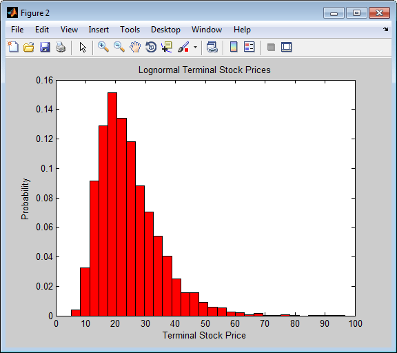
Display the sample density function of the terminal stock price after one calendar year. From the sample density function, the lognormal distribution of terminal stock prices is apparent.
[count, BinCenter] = hist(StockPrices(end,:), 30); figure bar(BinCenter, count/sum(count), 1,'r') xlabel('Terminal Stock Price') ylabel('Probability') title('Lognormal Terminal Stock Prices')
Input Arguments
Output Arguments
References
[1] Hull, J. C.Options, Futures, and Other Derivatives.Prentice-Hall, 2003.
Version History
Introduced before R2006a
You can also select a web site from the following list:
Americas
- América Latina(Español)
- Canada(English)
- United States(English)
Europe
- Belgium(English)
- Denmark(English)
- Deutschland(Deutsch)
- 西班牙(Español)
- Finland(English)
- France(Français)
- Ireland(English)
- Italia(Italiano)
- Luxembourg(English)
- Netherlands(English)
- Norway(English)
- Österreich(Deutsch)
- Portugal(English)
- Sweden(English)
- Switzerland
- United Kingdom(English)