秃顶

减少模型订单

在页面中崩溃

Syntax

[RSYS，INFO] = BALRED（SYS，订单）

[〜，info] = balred（sys）

[___] = balred（___，选择）

秃头（系统）

描述

example

[RSYS,info] = balred（系统,命令)computes a reduced-order approximationRSYSLTI模型系统。所需订单（状态数）由命令。您可以通过设置一次尝试多个订单命令到整数的向量，在这种情况下RSYSis an array of reduced models.秃顶还返回结构info还有其他信息，例如Hankel单数值（HSV），错误结合，正则化水平和Gramians的Cholesky因素。

example

[〜，info] = balred（系统)returns the structureinfowithout computing the reduced-order model. You can use this information to select the reduced order命令based on your desired fidelity.

Note

当性能是一个问题时，请避免通过使用从上述语法获得的信息选择所需的模型顺序，然后使用，然后使用RSYS = BALRED（SYS，订单，信息）计算还原级模型。

example

[___] = balred（___,opts)使用选项集计算还原模型opts您指定使用Balredoptions（控制系统工具箱）。您可以使用绝对和相对误差控制，强调某些时间或频段，并分离稳定且不稳定的模式来指定消除状态的其他选项。看Balredoptions（控制系统工具箱）创建和配置选项集opts。

example

秃顶(系统)在图上显示Hankel单数值和近似误差。利用hsvplot（控制系统工具箱）自定义此图。

例子

全部收缩

使用Hankel单数值降低订购模型

打开实时脚本

对于此示例，请使用Hankel单数值图选择合适的顺序并计算还原阶模型。

对于这种情况，生成具有40个状态的随机离散时间空间模型。

rng(0) sys = drss(40);

Plot the Hankel singular values using秃顶。

秃头（系统）

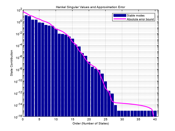
图包含一个轴对象。带有标题hankel单数值和近似错误的轴对象包含3个类型bar的对象。这些对象表示不稳定的模式，稳定模式，绝对错误绑定。

For this example, select order of16由于它是绝对错误的第一阶1E-4。In general, you select the order based on the desired absolute or relative fidelity. Then, compute the reduced-order model.

RSYS = BALRED（SYS，16）;

Verify the absolute error by plotting the singular value response usingsigma。

Sigma（SYS，SYS-RSYS）

图包含一个轴对象。The axes object contains 2 objects of type line. These objects represent sys, untitled1.

Observe from the plot that the error, represented by the red curve, is below-80 dB(1E-4）。

降级模型阵列

打开实时脚本

For this example, consider a random continuous-time state-space model with 65 states.

rng(0) sys = rss(65); size(sys)

具有1个输出，1个输入和65个状态的状态空间模型。

Visualize the Hankel singular values on a plot.

秃头（系统）

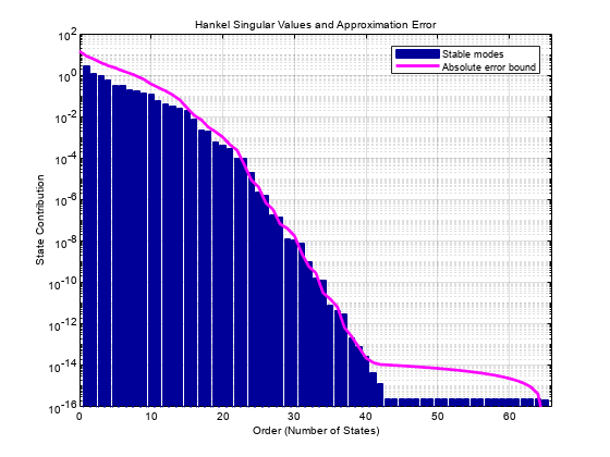
图包含一个轴对象。带有标题hankel单数值和近似错误的轴对象包含3个类型bar的对象。这些对象表示不稳定的模式，稳定模式，绝对错误绑定。

对于这种情况，计算25、30和35个状态的降级模型。

订单= [25,30,35];rsys = balred（sys，order）;尺寸（RSYS）

3x1状态空间模型阵列。每个模型都有1个输出，1个输入，在25至35个状态之间。

Reduced-Order Approximation with Offset Option

此示例使用：

控制系统工具箱控制系统工具箱

打开实时脚本

计算系统的降维近似m given by:

$G (s) = \frac{(s + 0 。 5) (s + 1 。 1) (s + 2 。 9)}{(s + 10^{- 6}) (s + 1) (s + 2) (s + 3)} 。$

创建模型。

sys = zpk（[ -  0.5 -1.1 -2.9]，[ -  1e -6 -2 -1 -3]，1）;

Exclude the pole at $s = 1 0^{- 6}$ 从稳定/不稳定分解的稳定项。为此，设置Offsetoption ofBalredoptions比您要排除的杆更大的值。

opts = balredoptions（'抵消'，0.001，'StateProjection','截短'）；

Visualize the Hankel singular values (HSV) and the approximation error.

BALRED（SYS，选择）

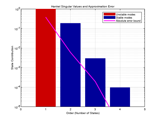
图包含一个轴对象。带有标题hankel单数值和近似错误的轴对象包含3个类型bar的对象。这些对象表示不稳定的模式，稳定模式，绝对错误绑定。

观察第一个HSV为红色，表明它与不稳定模式相关联。

Now, compute a second-order approximation with the specified options.

[rsys，info] = balred（sys，2，opts）;RSYS

RSYS= 0.99113 (s+0.5235) ------------------- (s+1e-06) (s+1.952) Continuous-time zero/pole/gain model.

Notice that the pole at-1E-6在还原模型中似乎没有变化RSYS。

比较原始模型和还原级模型的响应。

bodeplot(sys,rsys,'r-')

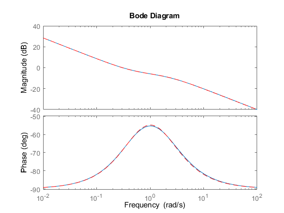
图包含2个轴对象。Axes object 1 contains 2 objects of type line. These objects represent sys, rsys. Axes object 2 contains 2 objects of type line. These objects represent sys, rsys.

观察原始模型的Bode响应和还原级模型几乎匹配。

Model Reduction in a Particular Frequency Band

此示例使用：

控制系统工具箱控制系统工具箱

打开实时脚本

减少高阶模型，重点是在特定频率范围内的动力学。

加载模型并检查其频率响应。

加载（'Highordormodel.mat','G'）BodePlot（G）

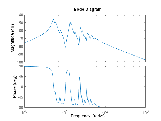
图包含2个轴对象。Axes object 1 contains an object of type line. This object represents G. Axes object 2 contains an object of type line. This object represents G.

G是一个第48阶模型，在5.2 rad/s，13.5 rad/s和24.5 rad/s之间具有几个大峰区域，并且散布在许多频率上的较小峰。假设对于您的应用，您只对第二个大峰附近的动力学感兴趣，即10 rad/s和22 rad/s。将模型降低集中在感兴趣区域，以获得与低阶近似的良好匹配。利用Balredoptions（控制系统工具箱）指定频率间隔秃顶。

bopt = balredoptions（'StateProjection','截短','freqintervals'，[10,22]）;glim10 = balred（g，10，bopt）;glim18 = balred（g，18，bopt）;

Examine the frequency responses of the reduced-order models. Also, examine the difference between those responses and the original response (the absolute error).

子图（2,1,1）;BodeMag（G，Glim10，Glim18，Logspace（0.5,1.5,100））;标题（“ bode幅度图”） 传奇（'原来的',订单10','订单18'）；subplot(2,1,2); bodemag(G-GLim10,G-GLim18,logspace(0.5,1.5,100)); title(“绝对错误图”） 传奇（订单10','订单18'）；

图包含2个轴对象。轴对象1包含3个类型行的对象。这些对象表示原始的，顺序10，顺序18。轴对象2包含2个类型行的对象。这些对象代表订单10，顺序18。

通过频率限制的能量计算，即使是10阶近似值也相当好。

Model-Order Reduction with Relative Error Approximation

打开实时脚本

对于此示例，请考虑SISO状态空间模型cdromwith 120 states. You can use absolute or relative error control when approximating models with秃顶。此示例比较将两种方法应用于便携式CD播放器设备的120状态模型crdom[1,2]。

加载CD播放器模型cdrom。

loadcdromdata.matcdromsize(cdrom)

具有1个输出，1个输入和120个状态的状态空间模型。

要将结果与绝对和相对错误控制的结果进行比较，请为每种方法创建一个选项集。

opt_abs = balredoptions（'错误键','绝对','StateProjection','truncate'）；opt_rel = balredoptions（'错误键','relative','StateProjection','truncate'）；

使用两种方法计算订单15的降级模型。

rsys_abs= balred(cdrom,15,opt_abs); rsys_rel = balred(cdrom,15,opt_rel); size(rsys_abs)

State-space model with 1 outputs, 1 inputs, and 15 states.

尺寸（rsys_rel）

State-space model with 1 outputs, 1 inputs, and 15 states.

Plot the Bode response of the original model along with the absolute-error and relative-error reduced models.

bo = bodeoptions;bo.posematching ='on';BodePlot（CDROM，'b.',rsys_abs,'r'，rsys_rel，'G'，bo）传奇（'Original (120 states)',“绝对错误（15个状态）”,'Relative Error (15 states)')

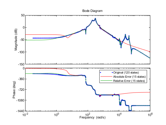
图包含2个轴对象。轴对象1包含3个类型行的对象。这些对象表示原始（120个状态），绝对错误（15个状态），相对误差（15个状态）。轴对象2包含3个类型行的对象。这些对象表示原始（120个状态），绝对错误（15个状态），相对误差（15个状态）。

Observe that the Bode response of:

相对纠正的模型rsys_rel几乎与原始模型的响应匹配系统在整个频率范围内。
绝对错误模型rsys_abs匹配原始模型的响应系统仅在收益最大的地区。

参考

降低模型的基准示例，系统和控制理论（slicot）中的子例程库。CDROM数据集经许可复制，请参阅BSD3-licensefor details.
A.Varga, “On stochastic balancing related model reduction”,Proceedings of the 39th IEEE Conference on Decision and Control (Cat. No.00CH37187)，悉尼，新南威尔士州，2000年，第2385-2390卷第3卷，doi：10.1109/cdc.2000.914156。

输入参数

全部收缩

`系统`—动态系统
动态系统模型

动态系统，指定为SISO或MIMO动态系统模型（控制系统工具箱）。您可以使用的动态系统可以是连续时间或离散时间数字LTI模型，例如TF,ZPK（控制系统工具箱），或者SS（控制系统工具箱）楷模。

什么时候系统has unstable poles,秃顶分解系统对于稳定且不稳定的零件，只有稳定的部分是近似的。利用Balredoptions（控制系统工具箱）to specify additional options for the stable/unstable decomposition.

秃顶不支持频率响应数据金宝app模型，不确定和广义状态空间模型，PID模型或稀疏模型对象。

`命令`—期望的状态数
整数|vector of integers

所需数量的状态，指定为整数或整数的向量。您可以通过设置一次尝试多个订单命令到整数的向量，在这种情况下rysis returned as an array of reduced models.

您还可以使用Hankel单数值和错误绑定信息来根据所需的模型保真度选择还原模型顺序。

`opts`—减少模型的其他选项
options set

减少模型的其他选项，指定为选项集。您可以使用绝对和相对误差控制，强调某些时间或频段，并分离稳定且不稳定的模式来指定消除状态的其他选项。

看Balredoptions（控制系统工具箱）创建和配置选项集opts。

输出参数

全部收缩

`RSYS`— Reduced-order model
动态系统模型| array of dynamic system models

Reduced-order model, returned as a dynamic system model or an array of dynamic system models.

`info`- 有关LTI模型的其他信息
结构体

有关LTI模型的其他信息，作为一个结构返回，具有以下字段：

HSV— Hankel singular values (state contributions to the input/output behavior). In state coordinates that equalize the input-to-state and state-to-output energy transfers, the Hankel singular values measure the contribution of each state to the input/output behavior. Hankel singular values are to model order what singular values are to matrix rank. In particular, small Hankel singular values signal states that can be discarded to simplify the model.
错误串- 在绝对或相对近似误差上绑定。info.errorbound（j+1）界限订单J的错误。
正则化- 正则化级别⍴（仅对相对误差）。这里，系统is replaced by[sys，⍴*i]或者[sys;⍴*i]这确保了所有频率下定义明确的相对误差。
RR,ro- Gramians的Cholesky因素。

算法

秃顶首先分解G进入其稳定且不稳定的部分：

$G = G_{s} + G_{u}$
指定时错误串as绝对,秃顶使用平衡的截断方法[1]to reduceG_s。这计算Hankel单数值（HSV）σ_j基于Gramians的可控性和可观察性。订单r，绝对错误 ${‖ G_{s} - G_{r} ‖}_{\infty}$ 受 $2 \sum_{j = r + 1}^{n} σ_{j}$ 。这里，n是在G_s。
指定时错误串asrelative,秃顶使用平衡的随机截断方法[2]to reduceG_s。对于正方形G_s, this computes the HSVσ_j相位矩阵 $F = {(W')}^{- 1} G$ 在哪里W(s)是稳定的最小光谱因子GG’:

$W' (s) W (s) = G (s) G' (s)$

订单r，相对错误 ${‖ G_{s}^{- 1} (G_{s} - G_{r}) ‖}_{\infty}$ 受:

$\prod_{j = r + 1}^{H} (\frac{1 + σ_{j}}{1 - σ_{j}}) - 1 \approx 2 \sum_{j = r + 1}^{n} σ_{j}$

什么时候， $2 \sum_{j = r + 1}^{n} σ_{j} ≪ 1$ 。

替代功能

应用程序

模型还原器（控制系统工具箱）

Live Editor Task

减少模型顺序（控制系统工具箱）

参考

[1] Varga，A。，“用于计算奇异扰动近似的无平衡方形 - 根 - 根算法”，”Proc. of 30th IEEE CDC，布莱顿，英国（1991），第1062-1065页。

[2] Green，M。，“平衡随机截断的相对误差”，IEEE Transactions on Automatic Control，卷。33，第10号，1988年

Version History

在R2006a之前引入

展开全部

R2017B：`matchdc`当指定频率或时间间隔不排除DC时，选项兑现

Behavior changed in R2017b

当您使用时秃顶为了减少模型，您可以使用Balredoptions（控制系统工具箱）将计算限制为指定的频率或时间间隔。如果是状态预选option ofBalredoptions被设定为'matchdc'（默认值），然后秃顶尝试匹配原始模型和简化模型的直流增益，即使指定的间隔排除了直流（频率= 0或time =inf）。

在R2017B之前，如果指定了不包括DC的时间或频率间隔，秃顶did not attempt to match the DC gain of the original and reduced models, even ifstate -procotion ='matchdc'。

看Also

Functions

Balredoptions（控制系统工具箱）

应用

模型还原器（控制系统工具箱）

Live Editor Tasks

减少模型顺序（控制系统工具箱）

Topics

模型还原基础（控制系统工具箱）
平衡截断模型还原（控制系统工具箱）

秃顶

Syntax

描述

例子

使用Hankel单数值降低订购模型

降级模型阵列

Reduced-Order Approximation with Offset Option

Model Reduction in a Particular Frequency Band

Model-Order Reduction with Relative Error Approximation

输入参数

系统—动态系统动态系统模型

命令—期望的状态数整数|vector of integers

opts—减少模型的其他选项options set

输出参数

RSYS— Reduced-order model动态系统模型| array of dynamic system models

info- 有关LTI模型的其他信息结构体

算法

替代功能

应用程序

Live Editor Task

参考

Version History

R2017B：matchdc当指定频率或时间间隔不排除DC时，选项兑现

看Also

Functions

应用

Live Editor Tasks

Topics

`系统`—动态系统
动态系统模型

`命令`—期望的状态数
整数|vector of integers

`opts`—减少模型的其他选项
options set

`RSYS`— Reduced-order model
动态系统模型| array of dynamic system models

`info`- 有关LTI模型的其他信息
结构体

R2017B：`matchdc`当指定频率或时间间隔不排除DC时，选项兑现