Optimize a pose graph based on the nodes and edge constraints. The pose graph used in this example is from theIntel Research Lab Datasetand was generated from collecting wheel odometry and a laser range finder sensor information in an indoor lab.

Load the Intel data set that contains a 2-D pose graph. Inspect theposeGraphobject to view the number of nodes and loop closures.

loadintel-2d-posegraph.matpgdisp(pg)

poseGraph with properties: NumNodes: 1228 NumEdges: 1483 NumLoopClosureEdges: 256 LoopClosureEdgeIDs: [1228 1229 1230 1231 1232 1233 1234 1235 1236 ... ] LandmarkNodeIDs: [1x0 double]

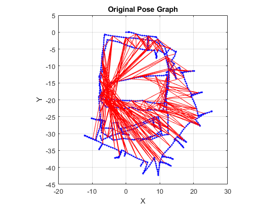
Plot the pose graph with IDs off. Red lines indicate loop closures identified in the dataset.

show(pg,'IDs','off'); title('Original Pose Graph')

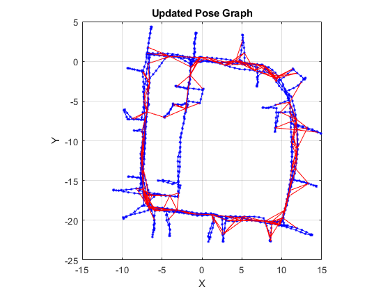
Optimize the pose graph. Nodes are adjusted based on the edge constraints and loop closures. Plot the optimized pose graph to see the adjustment of the nodes with loop closures.

updatedPG = optimizePoseGraph(pg); figure show(updatedPG,'IDs','off'); title('Updated Pose Graph')

Optimize a pose graph based on the nodes and edge constraints. The pose graph used in this example is taken from theMIT Datasetand was generated using information extracted from a parking garage.

Load the pose graph from the MIT dataset. Inspect theposeGraph3Dobject to view the number of nodes and loop closures.

loadparking-garage-posegraph.matpgdisp(pg);

poseGraph3Dwith properties: NumNodes: 1661 NumEdges: 6275 NumLoopClosureEdges: 4615 LoopClosureEdgeIDs: [128 129 130 132 133 134 135 137 138 139 140 ... ] LandmarkNodeIDs: [1x0 double]

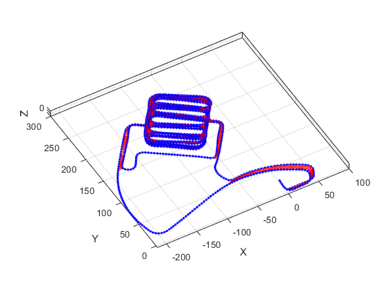
Plot the pose graph with IDs off. Red lines indicate loop closures identified in the dataset.

title('Original Pose Graph') show(pg,'IDs','off'); view(-30,45)

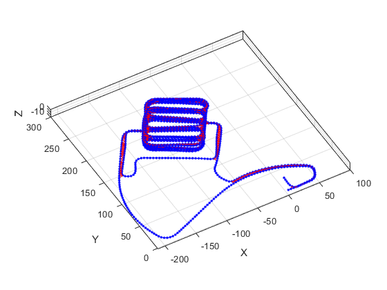
Optimize the pose graph. Nodes are adjusted based on the edge constraints and loop closures. Plot the optimized pose graph to see the adjustment of the nodes with loop closures.

updatedPG = optimizePoseGraph(pg); figure title('Updated Pose Graph') show(updatedPG,'IDs','off'); view(-30,45)