 Cleve’s Corner: Cleve Moler on Mathematics and Computing
 洛伦(Matlab)的艺术
 史蒂夫(Steve)与MATLAB进行图像处理
 家伙在simu金宝applink上
 deep Learning
 developer Zone
 Stuart的MATLAB视频
 头条新闻
头条新闻 档案交换一周
 Hans on IoT
 Student Lounge
 初创企业,加速器和企业家
 MATLAB社区
 MATLABユーザーコミュニティー
对称对分解
一个n esoteric fact about matrices is that any real matrix can be written as the product of two symmetric matrices. I've known about this fact for years, but never seriously explored the computational aspects. So I'm using this post to clarify my own understanding of what I'll call the对称对分解。It turns out that there are open questions. I don't think we know how to reliably compute the factors. But I also have to admit that, even if we could compute them, I don't know of any practical use.
内容
Theorem
没有多少人知道这个定理。
定理:任何实际矩阵都等于两个真实对称矩阵的乘积。
一个lmost Proof
乍一看,这定理智慧无关h eigenvalues. But here is the beginning of a proof, and a possible algorithm. Suppose that a real matrix $A$ has real, distinct eigenvalues. Then it can be diagonalized by the matrix $V$ of its eigenvectors.
$$A = V D V^{-1}$$
因为我们假设没有多个特征值,所以存在矩阵$ v $,并且是非词,并且矩阵$ d $是真实的和对角线的。让
$$ S_1 = V D V^T $$
$$ s_2 = v^{ - t} v^{ - 1} $$
然后$ s_1 $和$ s_2 $是真实的,对称的,它们的产品是
$$ S_1 S_2 = A $$
这个论点不是证明。它只是使定理合理。当矩阵重复特征值并且缺乏完整的特征向量时,挑战就会出现。一个完整的证明将将矩阵转换为其理性规范形式或其约旦规范形式,并以规范形式为块构建明确的对称因素。
自由程度
如果$ a $是$ n $ -by- $ n $,并且
$$ a = S_1 S_2 $$
where each of the symmetric matrices has $n(n+1)/2$ independent elements, then this is $n^2$ nonlinear equations in $n^2+n$ unknowns. It looks like there could be an $n$-parameter family of solutions. In my almost proof, each eigenvector is determined only up to a scale factor. These $n$ scale factors show up in $S_1$ and $S_2$ in complicated, nonlinear ways. I suspect that allowing complex scale factors parameterizes the complete set of solutions, but I'm not sure.
Moler's Rules
My two Golden Rules of computation are:
- 最难计算的事情是不存在的事物。
- 要计算的下一个最难的事情是不是唯一的事情。
对于对称对分解,我们晦涩的定理说分解存在,但是自由度观察的程度可能并非唯一。更糟糕的是,我们唯一需要的算法是可能不存在的全套特征向量。我们将不得不担心这些事情。
lu分解
数值线性代数中最重要的分解是我们用于求解同时线性方程系统的分解,是LU分解。它表示置换的矩阵作为两个三角因子的乘积。
$$ p a = l u $$
排列矩阵$ p $为我们提供了存在和数值稳定性。将$ l $的对角线放在对角线上,消除了$ n $ n $的自由度,并给我们带来独特性。
魔法广场
我们的第一个示例涉及我最喜欢的矩阵之一。
一个= magic(3)
a = 8 1 6 3 5 7 4 9 2
使用符号工具箱准确计算特征值和向量。
[v,d] = eig(sym(a))
v = [(2*6^(1/2))/5-7/5, - (2*6^(1/2))/5-7/5,1] [2/5 - (2*6^(1/2))/5,(2*6^(1/2))/5 + 2/5,1] [1,1,1] d = [-2*6^(1/2)),0,0] [0,2*6^(1/2),0] [0,0,15]
请注意,元素的元素v和d涉及$ \ sqrt {6} $,因此是非理性的。现在让
S1 =简化(V*D*V')S2 =简化(Inv(V*V'))
S1= [ 1047/25, -57/25, 27/5] [ -57/25, 567/25, 123/5] [ 27/5, 123/5, 15] S2 = [ 3/16, 1/12, 1/16] [ 1/12, 1/2, -1/4] [ 1/16, -1/4, 25/48]
$ \ sqrt {6} $消失了。你可以看到S1和S2是对称的,有理性的条目,正如宣传的那样,他们的产品是
Product = S1*S2
Product = [ 8, 1, 6] [ 3, 5, 7] [ 4, 9, 2]
让's play with the scale factors a bit. I particularly like
V(:,3)= 2 S1 =简化(V*D*V')/48 S2 = 48*Simplify(Inv(V*V'))
v = [(2*6^(1/2))/5-7/5, - (2*6^(1/2))/5-7/5,2] [2/5 - (2*6^(1/2))/5, (2*6^(1/2))/5 + 2/5, 2] [ 1, 1, 2] S1 = [ 181/100, 89/100, 21/20] [ 89/100, 141/100, 29/20] [ 21/20, 29/20, 5/4] S2 = [ 5, 0, -1] [ 0, 20, -16] [ -1, -16, 21]
现在S1has decimal fraction entries, andS2有整数条目,包括两个零。让我们离开象征世界。
s1 = double(s1)s2 = double(s2)product = s1*s2
S1 = 1.8100 0.8900 1.0500 0.8900 1.4100 1.4500 1.0500 1.4500 1.4500 1.2500 S2 = 5 0 -1 0 20 -16 -16 -16 21 21产品= 8 1 6 3 5 7 4 9 2
我不能保证通过其他示例获得如此漂亮的结果。
几乎有缺陷
假设我想计算约旦块的这种扰动的对称对分解。
e = sym('e',,,,'积极的');a = [2 1 0 0;0 2 1 0;0 0 2 1;E 0 0 2]
a = [2,1,0,0] [0,2,1,0] [0,0,2,1] [E,0,0,2]
这是特征值分解。向量已缩放,使最后一个分量等于1。特征值位于以2为中心的复合平面的圆上,半径为E^(1/4),,,,which is the signature of an eigenvalue of multiplicity 4.
[v,d] = eig(a);v =简化(v)d =简化(d)
v = [-i/e^(3/4),i/e^(3/4),1/e^(3/4),-1/e^(3/4)] [-1/e^(1/2),-1/e^(1/2),1/e^(1/2),1/e^(1/2)] [i/e^(1/4), -i/e^(1/4),1/e^(1/4),-1/e^(1/4)] [1,1,1,1,1] d = [2 -e^(1/4)*i,0,0,0] [0,e^(1/4)*i + 2,0,0] [0,0,e^(1/4) + 2,0] [0] [0] [0,0,0,2 -e^(1/4)]
这是该特征值分解产生的对称对分解。
s1 =简化(v*d*v。')s2 =简化(v*v.'))
s1 = [0,4/e,8/e,0] [4/e,8/e,0,0] [8/e,0,0,0,4] [0,0,0,4,8] s2 =[0,0,E/4,0] [0,E/4,0,0] [E/4,0,0,0,0] [0,0,0,0,1/4]
Well, this sort of does the job.S1和S2是对称的,它们的产品等于一个。
Product = S1*S2
product = [2,1,0,0] [0,2,1,0] [0,0,2,1] [E,0,0,2]
但是我担心这些因素的规模非常严重。我做的e较小,大元素S1get larger, and the small elements inS2get smaller. The decomposition breaks down.
更好的分解
更好的分解只是旋转。这两个矩阵是对称的,它们的产品是一个。
s2 = sym(rot90(眼睛(size(a))))s1 = a/s2 product = s1*s2
s2 = [0,0,0,1] [0,0,1,0] [0,1,0,0] [1,0,0,0,0] s1 = [0,0,0,1,2] [0,1,2,0] [1,2,0,0] [2,0,0,e] product = [2,1,0,0],2,1] [E,0,0,2]
我可以通过重新恢复特征向量来重现这种分解吗?这是使用符号求解功能来计算新的比例因素的代码。如果您想查看其工作原理,请在本文末尾使用链接下载此M文件,请删除本节中的分号,然后运行或发布再次。
s = sym(',[4,1]);v = v*diag(s);t =简化(Inv(v*v。'));soln = solve(t(:,1)-s2(:,1));s = [soln.s1(1);soln.s2(1);Soln.S3(1);Soln.S4(1)]
s =(e^(3/4)*i)^(1/2)/2(-e^(3/4)*i)^(1/2)/2 E^(3/8)/2(-e^(3/4))^(1/2)/2
These scale factors are complex numbers with magnitudeE^(3/8)/2。让我们重新汇总特征向量。当然,特征值不会改变。
[v,d] = eig(a);v =简化(v*diag(s))
v= [ -(-1)^(3/4)/(2*e^(3/8)), (-1)^(1/4)/(2*e^(3/8)), 1/(2*e^(3/8)), -i/(2*e^(3/8))] [ -(-1)^(1/4)/(2*e^(1/8)), -1/(-1)^(1/4)/(2*e^(1/8)), 1/(2*e^(1/8)), i/(2*e^(1/8))] [ ((-1)^(3/4)*e^(1/8))/2, -((-1)^(1/4)*e^(1/8))/2, e^(1/8)/2, -(e^(1/8)*i)/2] [ ((-1)^(1/4)*e^(3/8))/2, (1/(-1)^(1/4)*e^(3/8))/2, e^(3/8)/2, (e^(3/8)*i)/2]
现在,这些特征向量产生与旋转相同的稳定分解。
s1 =简化(v*d*v。')s2 =简化(v*v.'))
s1 = [0,0,1,2] [0,1,2,0] [1,2,0,0] [2,0,0,0,e] s2 = [0,0,0,0,0,1] [0,0,1,0] [0,1,0,0] [1,0,0,0,0]
可以小心地选择特征向量的缩放量表是声音数值算法的基础吗?我对此表示怀疑。我们仍在尝试使用几乎不存在的因素来计算并非唯一的东西。这真是摇摇欲坠。
- 类别:
- 矩阵


注释
要发表评论,请单击here登录您的数学帐户或创建一个新帐户。