 Cleve的角落:数学和计算上的Clyver
 Loren在Matlab的艺术上
 史蒂夫在图像处理与matlab
 Guy on Simulink
 深度学习
深度学习 开发人员区
开发人员区 Stuart的Matlab视频
 在头条新闻后面
 文件交换Pick of the Week
 汉斯在某地面
 Student Lounge
 Startups, Accelerators, & Entrepreneurs
 Matlab社区
 马铃薯草ユーザーコミュニティー
用预测警务战斗犯罪
我最近注意到有一个题为kaggle比赛旧金山犯罪分类这要求你预测犯罪t的类别hat occurred in San Franciso from 1/1/2003 to 5/13/2015 in theSFPD Crime Incident Reporting system. The goal of the competition is to predict the category of crime that occurred based on time and location.
这让我想起了电影Minority Report其中一个特殊的警察单位在犯罪之前逮捕人,但这是SciFi。一种更现实的方法是阻止犯罪通过分析过去的数据来预测犯罪何时以及将执法资源部署到此类热点。这种方法被称为predictive policing。

让我们来看看SFPD数据,看看我们可以从中学到什么。这与竞争对手的目标无关,但卡格是“also encouraging you to explore the dataset visually“. So why not?
Contents
SFPD犯罪事件报告数据
You need to first download the zipped data files from Kaggle website, unzip and place them into your current folder. Let’s load the data see what attributes are included.
t = readtable('train.csv'那'格式'那'%d%c%q%c%c%q%q%f%f'的);% load data from csvweek = {'Sunday'那'周一'那'周二'那'周三'那。。。%定义订单'Thursday'那'Friday'那'周六'};T.(4)= Reordercats(T.(4),周);%重新排序类别T.(6)=分类(T.(6));%转换为分类t.properties.variablenames.%显示变量名称
ans = Columns 1 through 5 'Dates' 'Category' 'Descript' 'DayOfWeek' 'PdDistrict' Columns 6 through 9 'Resolution' 'Address' 'X' 'Y'
让我们还添加一个新列来为特定的每周内Internvals分配日期以进行时间序列分析。
t = datetime('2003-1-5')+天(0:7:4515);%每周日期间隔weeks = NaT(size(T.Dates));%空日期时间数组为了i = 1:length(t) - 1% loop over weekly intervalsweeks(T.Dates >= t(i) & T.Dates < t(i+1)) = t(i);% dates to weekly intervals结尾T.Week = weeks;% add weekly intervals
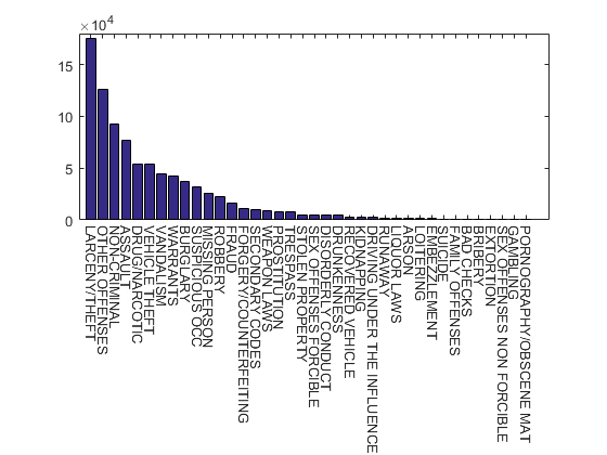
Now let’s see what is included in ‘Category’. There are 38 categories of crime and non-crime incidents, such as ARSON, ASSAULT, and BAD CHECKS, but which ones should we focus on?
t.category = mergecats(t.category,{'TRESPASS'那'trea'});% merge mislabeled categoriestab = tabulate(T.Category);%表格类别[Count, idx] = sort(cell2mat(tab(:,2)),“下降”的);% sort by category total数字% new figure酒吧(计数)%绘图条形图ax = gca;%获取当前轴柄ax.xtick = 1:尺寸(标签,1);%使用类别作为勾选ax.xticklabel =标签(IDX,1);%重命名刻度标签ax.XTickLabelRotation = -90;%垂直旋转文本
破坏窗口理论
这个理论那embraced by New York City Police Commissioner (then NYPD Chief)William Bratton在20世纪90年代,留下破碎的Windows未解档导致邻近的更加破坏和更大的社会疾病,因为它表示没有人在那里关心。达到那个点NYPD专注于解决严重的罪行。然而,该理论表明,在小型犯罪上开裂可能导致更严重的犯罪。虽然纽约在布塔隆下的犯罪率下降了,但这种理论并非没有批评者,因为它也导致了争议stop and frisk实践。
Perhaps this theory provides one starting point for our exploration. Does the SFPD data show a correlation between a petty crime like vandalism and other more serious crimes? Let’s start with bivariate histogram using直方图2to plot the vandalism incidents by location. Checksfcrime_load_map.。m看看如何从中检索栅格地图Web Map Service。
sfcrime_load_map.% load map from WMSvandalism = T(T.Category =='破坏者'那[1,3:5,8:10]);% subset T by categorynbins = 100;% number of binsxbinedges = linspace(lim.lon(1),lim.lon(2),nbins);%x bin边缘ybinedges = linspace(lim.lat(1),lim.lat(2),nbins);% y bin edges地图= flipud(a);%翻转图像数字% new figurecolormap凉爽的% set colormap直方图2(Vandalism.x,Vandalism.Y,。。。% plot 3D bivariatexbinedges, ybinedges,。。。% histogram'FaceColor'那'平坦的'那。。。'FaceAlpha',0.5,'Edgealpha',0.5)持有on%不要覆盖图像(lim.lon,lim.lat,地图)% add the map抓住off% 恢复默认ax = gca;%获取当前轴柄ax.clim = [0 100];% color axis scaling标题({'San Francisco Crime Map';。。。% 添加标题'Vandalism: Jan 2003 - May 2015'})zlabel('警察报告的计数'的)%添加轴标签文字(-122.52,37.82,300,'金门大桥'的)% annotate landmark文字(-122.4,37.82,200,'海湾大桥'的)% annotate landmark
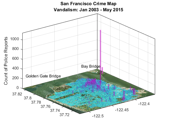
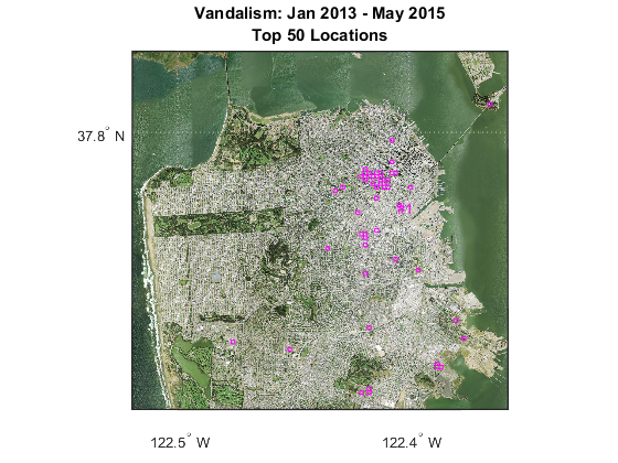
You can see that those incidents are highly concentrated in several hot spots indicated by the tall magenta bars. There is one particularly tall bar that sticks high above the rest. Where is it? We can plot the top 50 locations of high vandalism incidents with the highest spot marked as “#1”. Checksfcrime_draw_locs.m.to see the details.
数字% new figureUSAMAP(LIM.LAT,LIM.LON);% set map coordinatesGeoshow(A,R)%显示地图sfcrime_draw_locs(破坏,Lim.lat,Lim.lon,Nbins,50,'M'的)%画出前50个位置标题({'Vandalism: Jan 2013 - May 2015';'Top 50 Locations'})% 添加标题
犯罪热图
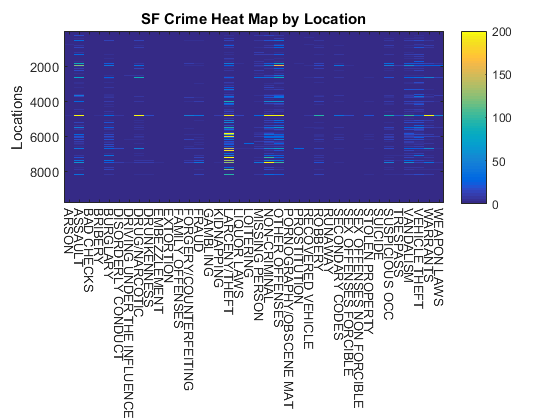
如果我们通过相同的网格处理其他类别的犯罪,我们可以通过位置创建犯罪矩阵,我们可以将其作为热图imagescto make comparison easier.
Bright horizontal stripes indicate a location where different types of crimes are committed. There is one particularly bright stripe with ASSAULT, DRUG/NARCOTIC, LARCENY/THEFT, NON-CRIMINAL, OTHER OFFENSES, and WARRANTS. ROBBERY, SUSPICIOUS OCC, and VANDALISM also appear in a lighter shade.
如果你看看盗窃/盗窃,它并不一定在它光明的地方形成条纹行。如果您要偷窃,那么要去找到高价值目标的地方可能是值得的。
CATS =类别(T.Category);%提取类别Rawcounts =零((nbins-1)^ 2,长度(猫));%设置累加器为了i = 1:length(cats)% loop over categoriesdata = t(t.category == cats {i},8:9);% subset T by category[N,~,~] = histcounts2(data.X, data.Y,。。。%获得双变量直方图Xbineges,Ybinedges);% bin countsrawCounts(:,i) = N(:);% add to accumulator结尾% as a vector数字% new figureimagesc(rawCounts)% plot matrix as an imageax = gca;%获取当前轴柄ax.clim = [0 200];% color axis scalingax.xtick = 1:长度(猫);%使用类别作为勾选ax.XTickLabel = cats;%重命名刻度标签ax.XTickLabelRotation = -90;%垂直旋转文本ylabel('Locations'的)%添加轴标签标题('SF犯罪热量地图按位置'的)% 添加标题彩色栏% add colorbar
Principal Components Analysis
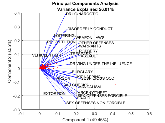
我们可以用Principal Component AnalysisuisngPCA.在不同类别中获得更好的关系并与结果相似双针。我们需要使用加权PCA来解决类别之间的大规模差异。我们还需要隐藏某些类别,因为如果我们尝试展示所有38个,输出将过于混乱。
w = 1 ./ var(rawCounts);%逆变量差异[WCOEFF,得分,潜伏,司干,解释] =。。。%加权PCA与wPCA(Rawcounts,'VariableWeights',w);coefforth = diag(sqrt(w))* wcoeff;% turn wcoeff to orthonormallabels = cats;% categories as labelslabels([4,9,10,12,13,15,18,20,21,23,25,27,28,31,32]) = {''};% drop some labels to avoid clutter数字% new figure双针(coefforth(:,1:2),'分数',得分(:,1:2),。。。% 2D biplot with the first two comps'VarLabels'那labels) xlabel(sprintf('Component 1 (%.2f%%)'那explained(1)))% add variance explained to x axis labelylabel(Sprintf('Component 2 (%.2f%%)'那explained(2)))%添加到y轴标签的方案轴([ - 0.1 0.6 -0.3 0.4]);%定义轴限制标题({'Principal Components Analysis';。。。% 添加标题Sprintf('方差解释%.2f %%',sum(解释(1:2)))})htext = findobj(gca,'String'那'VEHICLE THEFT'的);%找到文本对象htext.HorizontalAlignment ='right';%更改文本对齐htext = findobj(gca,'String'那'突击'的);%找到文本对象htext.position = [0.2235 0.0909 0];%移动标签位置htext = findobj(gca,'String'那'ROBBERY'的);%找到文本对象htext.position = [0.2148 0.1268 0];%移动标签位置htext = findobj(gca,'String'那'ARSON'的);%找到文本对象htext.HorizontalAlignment ='right';%更改文本对齐htext = findobj(gca,'String'那'EXTORTION'的);%找到文本对象htext.HorizontalAlignment ='right';%更改文本对齐
Assault, Robbery and Vehicle Theft
上半部分双针seems to show less sophisticated crimes than the lower half, and VANDALISM is more closely related to ARSON, and SUSPICIOUS OCC, and it is also related to LARCENY/THEFT but LARCENY/THEFT itself is closer to BAD CHECKS, EXTORTION, FRAUD and SEX OFFENSES FORCIBLE.
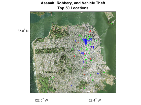
You can also see ASSAULT, ROBBERY, and VEHICLE THEFT are also very closely related. Among those, ASSAULT has the largest count of incidents. Maybe that’s the crime we need to focus on. Let’s check the top 50 locations for those crimes. As you would expect, you see good overlap of those locations.
assault = T(T.Category =='突击'那[1,3:5,8:10]);% subset T by category车辆= t(t.category =='VEHICLE THEFT'那[1,3:5,8:10]);% subset T by categoryrobbery = T(T.Category =='ROBBERY'那[1,3:5,8:10]);% subset T by category数字% new figureUSAMAP(LIM.LAT,LIM.LON);% set map coordinatesGeoshow(A,R)%显示地图TOPN = 50;%得到前50名抓住on%不要覆盖sfcrime_draw_locs(攻击,lim.lat,lim.lon,nbins,topn,'r'的)% draw locations in redsfcrime_draw_locs(vehicle,lim.lat,lim.lon,nbins,topN,'G'的)% draw locations in greensfcrime_draw_locs(抢劫,lim.lat,lim.lon,nbins,topn,'b'的)% draw locations in blue抓住off% 恢复默认标题({'Assault, Robbery, and Vehicle Theft';。。。% 添加标题Sprintf('top%d位置'那topN)})
Grand Theft Auto
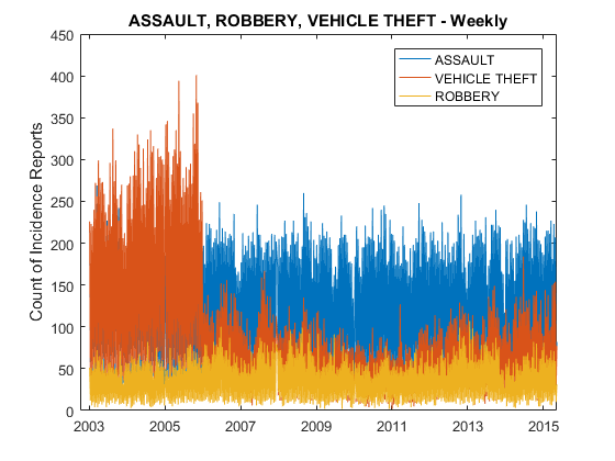
是否我们可以使用的数据预测,我们need to check the time dimension as well. We can use the weekly interval column to plot the weekly trends. This is strange. VEHICLE THEFT suddenly dropped in 2006! It’s time to dig deeper.
数字% new figure[g,t] = findgroups(assault.week);% group by weekly intervalsweekly = splitapply(@numel, assault.Week, G);%得到每周计数plot(t, weekly)%情节每周计数抓住on%不要覆盖(G, t) = findgroups (vehicle.Week);% group by weekly intervals每周= Splitapply(@numel,车辆。周,g);%得到每周计数plot(t, weekly)%情节每周计数[G, t] = findgroups(robbery.Week);% group by weekly intervals每周= Splitapply(@ numel,robbery.week,g);%得到每周计数plot(t, weekly)%情节每周计数抓住off% 恢复默认标题('攻击,抢劫,车辆盗窃 - 每周'的)% 添加标题ylabel('Count of Incidence Reports'的)%添加轴标签传奇('突击'那'VEHICLE THEFT'那'ROBBERY'的)% add legend
尤里卡!
Looking at descriptions, you notice that recovered vehicles are also reported as incidents. For some reason, it was the incidents of recovered vehicles that dropped off since 2006. Such a sudden change is usually caused by a change in reporting criteria, but it looks like half of the stolen cars were often recoveverd eventually in the good old days? Are they still recovered but not reported, or are they no longer recovered?This Boston Globe article提到“10辆车最常见的车辆,所有人都在2007年之前制作,”并获得了衰退的新的防盗装置,并说仍然被盗的人在海外发货(不可能被恢复)。
Anyhow, this time series analysis shows that there is a lot more going on than just time and location in crime. We could deal with the change in car theft reporting by omitting the data prior to 2006, but we would have to redo the heat map and run PCA again. Perhaps the Broken Windows Theory is not that useful as the basis of our analysis.
isRecovered = strfind(vehicle.Descript,'RECOVERED'的);% find 'RECOVERED' in descrptionisRecovered = ~cellfun(@(x) isempty(x), isRecovered);% is recovered if not empty[g,t] = findgroups(车辆。周(〜是isrocovered));% group by weekly intervalsweekly = splitapply(@numel, vehicle.Week(~isRecovered), G);%得到每周计数plot(t, weekly)%情节每周计数抓住on%不要覆盖[G, t] = findgroups(vehicle.Week(isRecovered));% group by weekly intervals每周= Splitapply(@numel,车辆。周(isrocovered),g);%得到每周计数plot(t, weekly)%情节每周计数抓住off% 恢复默认标题('VEHICLE THEFT - Weekly'的)% 添加标题ylabel('Count of Incidence Reports'的)%添加轴标签传奇('无人驾驶'那'RECOVERED'的)% add legend

另一种破碎的窗户
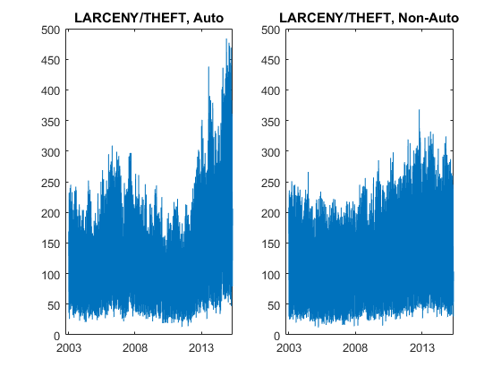
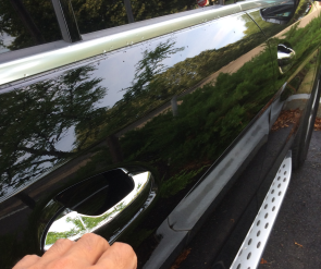
Loren分享了ny时代文章San Francisco Torn as Some See ‘Street Behavior’ Worsenwith me. It is about the rise of smash-and-grab thefts from vehicles from the perspective of a local resident at Lombard Street, famous for its zigzags. The article says victims are often tourists and out-of-town visitors. LARCENY/THEFT is clearly on the rise, and it indeed comes mainly from Auto-related thefts.
larceny = t(t.category =='LARCENY/THEFT'那[1,3:5,8:10]);% subset T by categoryisauto = strfind(larceny.descript,'LOCKED'的);% find 'LOCKED' in descrptionisauto =〜cellfun(@(x)isempty(x),isauto);%是自动的,如果不是空的数字% new figuresubplot(1,2,1)% subplot 1[g,t] = findgroups(larceny.week(Isauto));% group by weekly intervalsweekly = splitapply(@numel, larceny.Week(isAuto), G);%得到每周计数plot(t, weekly)%情节每周计数标题('盗窃/盗窃,自动'的)% 添加标题subplot(1,2,2)%子图2[G, t] = findgroups(larceny.Week(~isAuto));% group by weekly intervalsweekly = splitapply(@numel, larceny.Week(~isAuto), G);%得到每周计数plot(t, weekly)%情节每周计数标题('LARCENY/THEFT, Non-Auto'的)% 添加标题ylim([0 500])% adjust y-axis scale抓住off% 恢复默认
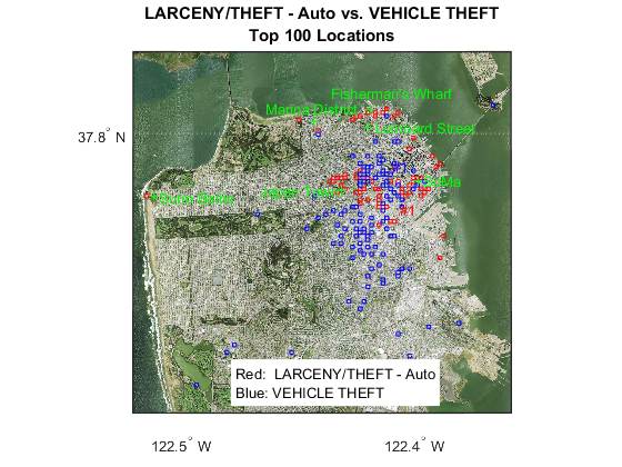
当您绘制与汽车相关的盗窃主/盗窃的前100个位置时,伦巴第街不会使剪切,但分布确实看起来与车辆盗窃不同。您可以看到渔夫码头和索马等着名旅游景点附近的几个地点,以其为科技公司的集中而闻名。似乎他们会在游客和商业历史记录不熟悉这片土地之后。现在我们发现影响一种犯罪的因素!
数字% new figureUSAMAP(LIM.LAT,LIM.LON);% set map coordinatesGeoshow(A,R)%显示地图TOPN = 100;% get top 100抓住on%不要覆盖sfcrime_draw_locs(larceny(isauto,:),lim.lat,lim.lon,。。。% draw locations in rednbins,topN,'r')SFCRIME_DRAW_LOCS(车辆,LIM.LAT,LIM.LON,NBINS,TOPN,'b'的)% draw locations in bluePlotm(37.802139,-122.41874,'+ g'的)% add landmarkplotm(37.808119, -122.41790,'+ g'的)% add landmarkPlotm(37.7808297,-122.4301075,'+ g'的)% add landmarkplotm(37.7842048, -122.3969652,'+ g'的)% add landmarkplotm(37.7786559, -122.5106296,'+ g'的)% add landmarkplotm(37.8038433, -122.4418518,'+ g'的)% add landmark抓住off% 恢复默认标题({'LARCENY/THEFT - Auto vs. VEHICLE THEFT';。。。% 添加标题Sprintf('top%d位置',topn)})Textm(37.802139,-122.41574,'Lombard Street'那。。。% annotate landmark'颜色'那'G') textm (37.814118.7.那-122.43450,'渔人码头'那。。。% annotate landmark'颜色'那'G'的)textm(37.7808297, -122.4651075,'日本小镇'那。。。% annotate landmark'颜色'那'G'的)textm(37.7842048, -122.3949652,'SoMa'那。。。% annotate landmark'颜色'那'G'的)textm(37.7786559, -122.5086296,'Sutro Baths'那。。。% annotate landmark'颜色'那'G')Textm(37.8088629,-122.4628518,'Marina District'那。。。% annotate landmark'颜色'那'G')Textm(37.715564,-122.475662,。。。%添加注意{'Red: LARCENY/THEFT - Auto'那'Blue: VEHICLE THEFT'},'背景颜色'那'w'的)
Summary
We looked at the Broken Windows Theory as a starting point of this exploration, but the SFPD data doesn’t provide easily detectable correlation among crimes that you would expect based on this theory, and time series analysis shows that there is a lot more going on than just time and location that affects crime. When we focused on specific types of crime that are in decline or on the rise, and cross referenced those with external data sources, we learned a lot more. This points to a potential for enriching this dataset with data from other sources like demographics to improve predictive capability, but it also creates违法行为的困境if not done carefully. British Transit Police got creative and did an interesting experiment to放置“看着眼睛”海报来阻止自行车盗窃。这是一种良好的创造性地利用这类分析的洞察力。
顺便说一下,我忍不住玩耍Matlab图形中的相机对象。这是旧金山犯罪现场的有趣跨桥动画!退房sfcrime_flyover.m为了more details.

Hopefully you now see how you can fight crime with data. Download this post in standard MATLAB script (click “_Get the MATLAB code_” below) and use it as the starting point for your exploration or even join Kaggle competition. If you find anything interesting, please let us know!
发布了MATLAB®R2016A
- Category:
- 社交计算


也可以看看
-
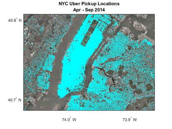
在纽约市映射Uber皮卡
博客


Comments
To leave a comment, please click这里to sign in to your MathWorks Account or create a new one.