基于深度学习的多光谱图像语义分割

这个示例使用:

打开生活的脚本

这个例子展示了如何使用U-Net对一个有七个通道的多光谱图像进行语义分割。

语义分割包括用类标记图像中的每个像素。语义分割的一个应用是跟踪森林砍伐，即森林覆盖随时间的变化。环境机构跟踪森林砍伐，以评估和量化一个地区的环境和生态健康。

基于深度学习的语义分割可以从高分辨率航空照片中获得精确的植被覆盖测量值。一个挑战是区分具有相似视觉特征的类别，例如试图将绿色像素划分为草、灌木或树。为了提高分类精度，一些数据集包含多光谱图像，提供关于每个像素的额外信息。例如，哈姆林海滩州立公园的数据集用三个近红外通道补充了彩色图像，提供了更清晰的分类。

这个例子展示了如何使用基于深度学习的语义分割技术从一组多光谱图像中计算一个区域的植被覆盖百分比。

下载数据

本例使用高分辨率多光谱数据集对网络进行训练[1]．在哈姆林海滩州立公园，纽约哈林海滩州立公园的无人机捕获了图像集。数据包含标记为培训，验证和测试集，具有18个对象类标签。数据文件的大小为3.0 GB。

下载数据集的MAT-file版本downloadHamlinBeachMSIDatahelper函数。这个函数作为支持文件附加到示例中。金宝app

imageDir = tempdir;url =“http://www.cis.rit.edu/ ~ rmk6217 / rit18_data.mat”；downloadHamlinBeachMSIData (url, imageDir);

检查训练数据

将数据集加载到工作区中。

负载(fullfile (imageDir“rit18_data”，“rit18_data.mat”））;

检查数据的结构。

谁train_dataval_datatest_data

Name Size Bytes Class Attributes test_data 7x12446x7654 1333663576 uint16 train_data 7x9393x5642 741934284 uint16 val_data 7x8833x6918 855493716 uint16

多光谱图像数据排列为numChannels——- - - - - -宽度——- - - - - -高度数组。而在MATLAB®中，多通道图像排列为宽度——- - - - - -高度——- - - - - -numChannels数组。要重塑数据以使通道处于第三维，请使用助手函数，switchChannelsToThirdPlane．这个函数作为支持文件附加到示例中。金宝app

train_data = switchChannelsToThirdPlane (train_data);val_data = switchChannelsToThirdPlane (val_data);test_data = switchChannelsToThirdPlane (test_data);

确认数据具有正确的结构。

谁train_dataval_datatest_data

Name Size Bytes Class Attributes test_data 12446x7654x7 1333663576 uint16 train_data 9393x5642x7 741934284 uint16 val_data 8833x6918x7 855493716 uint16

RGB颜色通道是第3、2和1个图像通道。以蒙太奇的形式显示训练、验证和测试图像的颜色组件。要使图像在屏幕上显得更亮，可以使用histeq(图像处理工具箱)函数。

图蒙太奇(．..{histeq (train_data (:,: [3 2 1])),．..histeq (val_data (:,:, (3 2 1))),．..histeq (test_data (:,:, (3 2 1)))},．..“BorderSize”10“写成BackgroundColor”，“白色”)标题(“训练图像(左)、验证图像(中)和测试图像(右)的RGB组件”）

以蒙太奇的形式显示训练数据的最后三个直方图均衡化通道。这些通道对应于近红外波段，并根据它们的热信号突出图像的不同组成部分。例如，靠近第二个通道图像中心的树比其他两个通道中的树显示更多的细节。

图蒙太奇(．..{histeq (train_data (:: 4)),．..histeq (train_data (:: 5)),．..histeq (train_data (:: 6))},．..“BorderSize”10“写成BackgroundColor”，“白色”)标题('IR频道1（左），2，（中心）和3（右）的训练图像'）

通道7是一个表示有效分割区域的掩码。显示训练、验证和测试图像的掩码。

图蒙太奇(．..{train_data (:: 7)．..val_data (:: 7)．..test_data (:: 7)},．..“BorderSize”10“写成BackgroundColor”，“白色”)标题(“训练图像遮罩(左)、验证图像(中)和测试图像(右)”）

标记的图像包含用于分割的ground truth数据，每个像素被分配到18个类中的一个。获取具有相应id的类的列表。

disp(类)

0.其他类/图像边界路标2。树3。建设4。交通工具(汽车、卡车或公共汽车)6人。救生员椅7。野餐的好表8。9.黑色木板 White Wood Panel 10. Orange Landing Pad 11. Water Buoy 12. Rocks 13. Other Vegetation 14. Grass 15. Sand 16. Water (Lake) 17. Water (Pond) 18. Asphalt (Parking Lot/Walkway)

创建一个包含类名的向量。

一会= [“路标”，“树”，“建筑”，“汽车”，“人”，．..“LifeguardChair”，“PicnicTable”，“BlackWoodPanel”，．..“WhiteWoodPanel”，“OrangeLandingPad”，“浮”，“石头”，．..“LowLevelVegetation”，“Grass_Lawn”，“Sand_Beach”，．..“Water_Lake”，“Water_Pond”，“沥青”]；

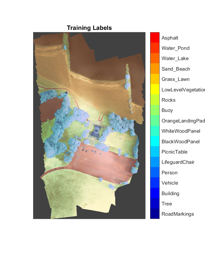
在直方图均衡化的RGB训练图像上叠加标签。给图像添加一个颜色条。

提出=喷气(元素个数(类名);B = labeloverlay (histeq (train_data (:,: 4:6)), train_labels,'透明度'，0.8，“Colormap”,提出);图imshow (B)标题(“培训”标签) N = numel(classNames);蜱虫= 1 / (N * 2): 1 / N: 1;colorbar (“TickLabels”cellstr(类名),“滴答”蜱虫,“TickLength”0,“TickLabelInterpreter”，“没有”）;colormap城市规划机构(cmap)

将培训数据保存为MAT文件，将培训标签保存为PNG文件。

保存(“train_data.mat”，“train_data”）;imwrite (train_labels“train_labels.png”）;

创建用于训练的随机补丁提取数据存储

使用随机补丁提取数据存储将训练数据提供给网络。该数据存储从包含地面真像和像素标签数据的图像数据存储和像素标签数据存储中提取多个相应的随机patch。打补丁是一种常见的技术，可以防止大图像内存耗尽，并有效地增加可用的训练数据量。

从存储训练图像开始“train_data.mat”在一个imageDatastore．因为MAT文件格式是非标准的图像格式，所以必须使用MAT文件阅读器来读取图像数据。你可以使用辅助MAT文件读取器，matReader，从训练数据中提取前6个通道，并省略包含掩码的最后一个通道。这个函数作为支持文件附加到示例中。金宝app

imd = imageDatastore (“train_data.mat”，“FileExtensions”，“.mat”，“ReadFcn”, @matReader);

创建一个pixelLabelDatastore(计算机视觉工具箱)存储包含18个已标记区域的标签补丁。

pixelLabelIds = 1:18;pxds = pixelLabelDatastore (“train_labels.png”一会,pixelLabelIds);

创建一个randomPatchExtractionDatastore(图像处理工具箱)从图像数据存储和像素标签数据存储。每个小批量包含16个256 × 256像素的补丁。在历元的每个迭代中提取1000个小批量。

pxds dsTrain = randomPatchExtractionDatastore (imd, [256256],“PatchesPerImage”, 16000);

随机补丁提取数据存储dsTrain在epoch的每次迭代中向网络提供小批量的数据。预览数据存储以探索数据。

inputBatch =预览(dsTrain);disp (inputBatch)

InputImage ResponsePixelLabelImage  __________________ _______________________ { 256×256×6 uint16}{256×256分类}{256×256×6 uint16}{256×256分类}{256×256×6 uint16}{256×256分类}{256×256×6 uint16}{256×256分类}{256×256×6 uint16}{256×256分类}{256×256×6 uint16}{256×256分类}{256×256×6 uint16}{256×256 categorical} {256×256×6 uint16} {256×256 categorical}

创建U-Net网络层

本例使用U-Net网络的一种变体。在U-Net中，最初的卷积层序列被最大池化层点缀，依次降低了输入图像的分辨率。这些层之后是一系列交错上采样算子的卷积层，依次提高了输入图像的分辨率[2]．U- net这个名字来源于这样一个事实:这个网络可以被画成一个像字母U一样的对称形状。

本例修改了U-Net，使其在卷积中使用零填充，以便卷积的输入和输出具有相同的大小。使用辅助函数，createUnet，创建一个带有一些预先选择的超参数的U-Net。这个函数作为支持文件附加到示例中。金宝app

inputTileSize = (256256 6);lgraph = createUnet (inputTileSize);disp (lgraph.Layers)

58×1图层数组:1“ImageInputLayer”图像输入图像256×256×6”zerocenter正常化2 Encoder-Section-1-Conv-1卷积64 3×3×6旋转步[1]和填充[1 1 1 1]3‘Encoder-Section-1-ReLU-1 ReLU ReLU 4 Encoder-Section-1-Conv-2卷积64 3×3×64旋转步[1]和填充(1 1 1)5‘Encoder-Section-1-ReLU-2 ReLU ReLU 6“Encoder-Section-1-MaxPool”马克斯池2×2马克斯池步(2 - 2)和填充[0 0 0 0]7 Encoder-Section-2-Conv-1卷积128 3×3×64旋转步[1]和填充(1 1 1)8“Encoder-Section-2-ReLU-1”ReLU ReLU 9 Encoder-Section-2-Conv-2卷积128 3×3×128旋转步[1]和填充[1 1 1 1]10“Encoder-Section-2-ReLU-2”ReLU ReLU 11“Encoder-Section-2-MaxPool”马克斯池2×2马克斯池步[2 2]和填充[0 0 0 0]12 Encoder-Section-3-Conv-1卷积256 3×3×128旋转步[1]和填充[1 1 1 1]13“Encoder-Section-3-ReLU-1”ReLU ReLU 14“Encoder-Section-3-Conv-2”Convolution 256 3×3×256 convolutions with stride [1 1] and padding [1 1 1 1] 15 'Encoder-Section-3-ReLU-2' ReLU ReLU 16 'Encoder-Section-3-MaxPool' Max Pooling 2×2 max pooling with stride [2 2] and padding [0 0 0 0] 17 'Encoder-Section-4-Conv-1' Convolution 512 3×3×256 convolutions with stride [1 1] and padding [1 1 1 1] 18 'Encoder-Section-4-ReLU-1' ReLU ReLU 19 'Encoder-Section-4-Conv-2' Convolution 512 3×3×512 convolutions with stride [1 1] and padding [1 1 1 1] 20 'Encoder-Section-4-ReLU-2' ReLU ReLU 21 'Encoder-Section-4-DropOut' Dropout 50% dropout 22 'Encoder-Section-4-MaxPool' Max Pooling 2×2 max pooling with stride [2 2] and padding [0 0 0 0] 23 'Mid-Conv-1' Convolution 1024 3×3×512 convolutions with stride [1 1] and padding [1 1 1 1] 24 'Mid-ReLU-1' ReLU ReLU 25 'Mid-Conv-2' Convolution 1024 3×3×1024 convolutions with stride [1 1] and padding [1 1 1 1] 26 'Mid-ReLU-2' ReLU ReLU 27 'Mid-DropOut' Dropout 50% dropout 28 'Decoder-Section-1-UpConv' Transposed Convolution 512 2×2×1024 transposed convolutions with stride [2 2] and cropping [0 0 0 0] 29 'Decoder-Section-1-UpReLU' ReLU ReLU 30 'Decoder-Section-1-DepthConcatenation' Depth concatenation Depth concatenation of 2 inputs 31 'Decoder-Section-1-Conv-1' Convolution 512 3×3×1024 convolutions with stride [1 1] and padding [1 1 1 1] 32 'Decoder-Section-1-ReLU-1' ReLU ReLU 33 'Decoder-Section-1-Conv-2' Convolution 512 3×3×512 convolutions with stride [1 1] and padding [1 1 1 1] 34 'Decoder-Section-1-ReLU-2' ReLU ReLU 35 'Decoder-Section-2-UpConv' Transposed Convolution 256 2×2×512 transposed convolutions with stride [2 2] and cropping [0 0 0 0] 36 'Decoder-Section-2-UpReLU' ReLU ReLU 37 'Decoder-Section-2-DepthConcatenation' Depth concatenation Depth concatenation of 2 inputs 38 'Decoder-Section-2-Conv-1' Convolution 256 3×3×512 convolutions with stride [1 1] and padding [1 1 1 1] 39 'Decoder-Section-2-ReLU-1' ReLU ReLU 40 'Decoder-Section-2-Conv-2' Convolution 256 3×3×256 convolutions with stride [1 1] and padding [1 1 1 1] 41 'Decoder-Section-2-ReLU-2' ReLU ReLU 42 'Decoder-Section-3-UpConv' Transposed Convolution 128 2×2×256 transposed convolutions with stride [2 2] and cropping [0 0 0 0] 43 'Decoder-Section-3-UpReLU' ReLU ReLU 44 'Decoder-Section-3-DepthConcatenation' Depth concatenation Depth concatenation of 2 inputs 45 'Decoder-Section-3-Conv-1' Convolution 128 3×3×256 convolutions with stride [1 1] and padding [1 1 1 1] 46 'Decoder-Section-3-ReLU-1' ReLU ReLU 47 'Decoder-Section-3-Conv-2' Convolution 128 3×3×128 convolutions with stride [1 1] and padding [1 1 1 1] 48 'Decoder-Section-3-ReLU-2' ReLU ReLU 49 'Decoder-Section-4-UpConv' Transposed Convolution 64 2×2×128 transposed convolutions with stride [2 2] and cropping [0 0 0 0] 50 'Decoder-Section-4-UpReLU' ReLU ReLU 51 'Decoder-Section-4-DepthConcatenation' Depth concatenation Depth concatenation of 2 inputs 52 'Decoder-Section-4-Conv-1' Convolution 64 3×3×128 convolutions with stride [1 1] and padding [1 1 1 1] 53 'Decoder-Section-4-ReLU-1' ReLU ReLU 54 'Decoder-Section-4-Conv-2' Convolution 64 3×3×64 convolutions with stride [1 1] and padding [1 1 1 1] 55 'Decoder-Section-4-ReLU-2' ReLU ReLU 56 'Final-ConvolutionLayer' Convolution 18 1×1×64 convolutions with stride [1 1] and padding [0 0 0 0] 57 'Softmax-Layer' Softmax softmax 58 'Segmentation-Layer' Pixel Classification Layer Cross-entropy loss

选择培训选项

训练网络使用随机梯度下降与动量(SGDM)优化。方法指定SGDM的超参数设置trainingOptions函数。

训练一个深度网络是非常耗时的。通过指定高学习率来加速训练。然而，这可能会导致网络的梯度发生爆炸或无法控制地增长，从而阻碍网络的成功训练。要使渐变保持在有意义的范围内，可以通过指定来启用渐变剪辑'gradientthreshold'作为0．05,并指定“GradientThresholdMethod”使用梯度的L2-norm。

initialLearningRate = 0.05;maxEpochs = 150;minibatchSize = 16;l2reg = 0.0001;选择= trainingOptions (“个”，．..'italllearnrate'initialLearningRate,．..'势头', 0.9,．..“L2Regularization”l2reg,．..“MaxEpochs”maxEpochs,．..“MiniBatchSize”minibatchSize,．..“LearnRateSchedule”，“分段”，．..“洗牌”，“every-epoch”，．..“GradientThresholdMethod”，“l2norm”，．..'gradientthreshold', 0.05,．..“阴谋”，“训练进步”，．..“VerboseFrequency”, 20);

培训网络

默认情况下，示例使用downloadTrainedUnethelper函数。这个函数作为支持文件附加到示例中。金宝app预先训练过的网络使您能够运行整个示例，而不必等待训练完成。

要训练网络，请设置doTraining变量为真正的．使用。训练模型Trainnetwork.函数。

在可用的GPU上进行训练。使用GPU需要并行计算工具箱™和支持CUDA®的NVIDIA®GPU。有关更多信息，请参见GPU支金宝app持情况(并行计算工具箱)．在NVIDIA Titan X上训练大约需要20个小时。

doTraining = false;如果doTraining [net,info] = trainNetwork(dsTrain,lgraph,options);modelDateTime =字符串(datetime (“现在”，“格式”，“yyyy-MM-dd-HH-mm-ss”））;保存(strcat (“multispectralUnet——”modelDateTime,“时代——”num2str (maxEpochs),“.mat”），“净”）;别的trainedUnet_url =“//www.tatmou.com/金宝appsupportfiles/vision/data/multispectralUnet.mat”；downloadTrainedUnet (trainedUnet_url imageDir);负载(fullfile (imageDir“trainedUnet”，'multispectralunet.mat'））;结束

现在可以使用U-Net对多光谱图像进行语义分割。

预测测试数据的结果

要在经过训练的网络上执行前向传递，请使用辅助函数，segmentImage，使用验证数据集。这个函数作为支持文件附加到示例中。金宝appsegmentImage的方法对图像块进行分割semanticseg(计算机视觉工具箱)函数。

predictPatchSize = [1024 1024];segmentedImage = segmentImage (val_data,净,predictPatchSize);

为了只提取分割的有效部分，将分割后的图像乘以验证数据的掩模通道。

segmentedImage = uint8(val_data(:，:，7)~=0) .* segmentedImage;图imshow (segmentedImage,[])标题(“分割图像”）

语义分割的输出是有噪声的。执行后期图像处理以去除噪声和杂散像素。使用medfilt2(图像处理工具箱)函数去除分割中的椒盐噪声。可视化的分割图像与噪声去除。

semmentedimage = medfilt2（sementedimage，[7,7]）;imshow（segmentedimage，[]）;标题（'被删除的噪音分段图像'）

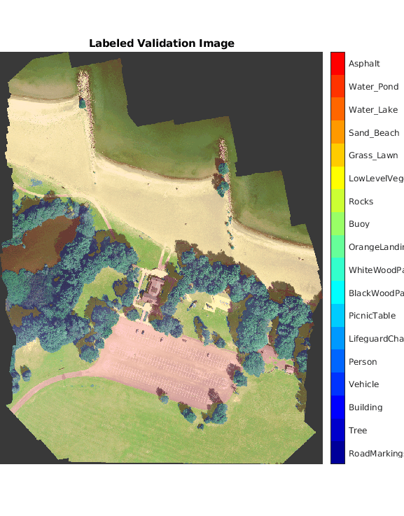
将分割后的图像叠加到直方图均衡化的RGB验证图像上。

B = labeloverlay(histeq(val_data(:，:，[3 2 1]))，segmentedImage，'透明度'，0.8，“Colormap”,提出);图imshow (B)标题(“标记验证图像”) colorbar (“TickLabels”cellstr(类名),“滴答”蜱虫,“TickLength”0,“TickLabelInterpreter”，“没有”）;colormap城市规划机构(cmap)

将分割后的图像和ground truth标签保存为PNG文件。这些将用于计算精度度量。

imwrite (segmentedImage“results.png”）;imwrite (val_labels“gtruth.png”）;

量化细分精度

创建一个pixelLabelDatastore(计算机视觉工具箱)为分割结果和地面真值标签。

pxdsResults = pixelLabelDatastore (“results.png”一会,pixelLabelIds);pxdsTruth = pixelLabelDatastore (“gtruth.png”一会,pixelLabelIds);

用该方法对语义切分的全局精度进行度量evaluateSemanticSegmentation(计算机视觉工具箱)函数。

ssm = evaluateManticStimation（PXDSResults，pxdstruth，“指标”，“global-accuracy”）;

评估语义分割结果  ---------------------------------------- * 所选指标:全球精度。*处理1幅图像。*完成……完成了。*数据集指标:GlobalAccuracy ______________ 0.90698

总体精度评分表明，只有超过90%的像素被正确分类。

计算植被覆盖范围

该示例的最终目标是计算多光谱图像中植被覆盖的程度。

找到标记植被的像素数。标签id 2(“Trees”)、13(“LowLevelVegetation”)和14(“Grass_Lawn”)是植被类。并通过对掩模图像感兴趣区域内像素的求和得到有效像素的总数。

vegetationClassIds = uint8([2、13、14]);vegetationPixels = ismember (segmentedImage (:), vegetationClassIds);validPixels = (segmentedImage ~ = 0);numVegetationPixels =总和(vegetationPixels (:));numValidPixels =总和(validPixels (:));

用植被像元数除以有效像元数来计算植被覆盖的百分比。

percentVegetationCover = (numVegetationPixels / numValidPixels) * 100;流(“植被覆盖百分比是%3.2f%%。”, percentVegetationCover);

植被覆盖率为51.72%。

参考文献

R. Kemker, C. Salvaggio和C. Kanan。用于语义分割的高分辨率多光谱数据集。, abs / 1703.01918。2017.

Ronneberger, O.， P. Fischer和T. Brox。U-Net:用于生物医学图像分割的卷积网络。, abs / 1505.04597。2015.

另请参阅

外部网站

https://github.com/rmkemker/RIT-18