Assess EGARCH Forecast Bias Using Simulations
这个例子展示了如何模拟EGARCH过程ss. Simulation-based forecasts are compared to minimum mean square error (MMSE) forecasts, showing the bias in MMSE forecasting of EGARCH processes.
Specify an EGARCH model.
Specify an EGARCH(1,1) process with constant , GARCH coefficient , ARCH coefficient and leverage coefficient .
Mdl = egarch('Constant',0.01,'GARCH',0.7,...'ARCH',0.3,'Leverage',-0.1)
Mdl = egarch with properties: Description: "EGARCH(1,1) Conditional Variance Model (Gaussian Distribution)" Distribution: Name = "Gaussian" P: 1 Q: 1 Constant: 0.01 GARCH: {0.7} at lag [1] ARCH: {0.3} at lag [1] Leverage: {-0.1} at lag [1] Offset: 0
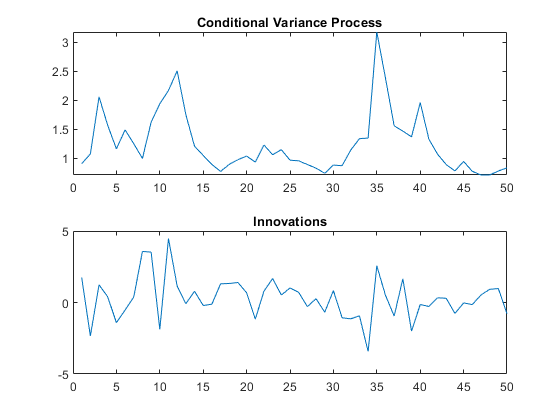
Simulate one realization.
Simulate one realization of length 50 from the EGARCH conditional variance process and corresponding innovations.
rngdefault;% For reproducibility[v,y] = simulate(Mdl,50); figure subplot(2,1,1) plot(v) xlim([0,50]) title('Conditional Variance Process') subplot(2,1,2) plot(y) xlim([0,50]) title(“创新”)
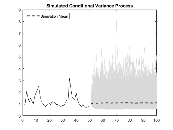
Simulate multiple realizations.
Using the generated conditional variances and innovations as presample data, simulate 5000 realizations of the EGARCH process for 50 future time steps. Plot the simulation mean of the forecasted conditional variance process.
rngdefault;% For reproducibility[Vsim,Ysim] = simulate(Mdl,50,'NumPaths',5000,...'E0',y,'V0',v); figure plot(v,'k') holdonplot(51:100,Vsim,'Color',[.85,.85,.85]) xlim([0,100]) h = plot(51:100,mean(Vsim,2),'k--','LineWidth',2); title('Simulated Conditional Variance Process') legend(h,'Simulation Mean','Location','NorthWest') holdoff
Compare simulated and MMSE conditional variance forecasts.
Compare the simulation mean variance, the MMSE variance forecast, and the exponentiated, theoretical unconditional log variance.
The exponentiated, theoretical unconditional log variance for the specified EGARCH(1,1) model is
sim = mean(Vsim,2); fcast = forecast(Mdl,50,y,'V0',v); sig2 = exp(0.01/(1-0.7)); figure plot(sim,':','LineWidth',2) holdonplot(fcast,'r','LineWidth',2) plot(ones(50,1)*sig2,'k--','LineWidth',1.5) legend('Simulated','MMSE','Theoretical') title('Unconditional Variance Comparisons') holdoff
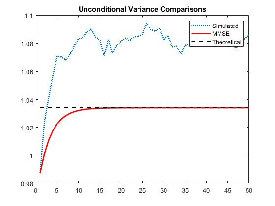
The MMSE and exponentiated, theoretical log variance are biased relative to the unconditional variance (by about 4%) because by Jensen's inequality,
Compare simulated and MMSE log conditional variance forecasts.
Compare the simulation mean log variance, the log MMSE variance forecast, and the theoretical, unconditional log variance.
logsim = mean(log(Vsim),2); logsig2 = 0.01/(1-0.7); figure plot(logsim,':','LineWidth',2) holdonplot(log(fcast),'r','LineWidth',2) plot(ones(50,1)*logsig2,'k--','LineWidth',1.5) legend('Simulated','MMSE','Theoretical') title('Unconditional Log Variance Comparisons') holdoff
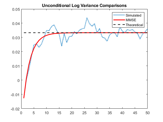
The MMSE forecast of the unconditional log variance is unbiased.
See Also
Objects
Functions
相关的例子
More About
Select a Web Site
Choose a web site to get translated content where available and see local events and offers. Based on your location, we recommend that you select:.
Selectweb siteYou can also select a web site from the following list:
Americas
- América Latina(Español)
- Canada(English)
- United States(English)
Europe
- Belgium(English)
- Denmark(English)
- Deutschland(Deutsch)
- España(Español)
- Finland(English)
- France(Français)
- Ireland(English)
- Italia(Italiano)
- Luxembourg(English)
- Netherlands(English)
- Norway(English)
- Österreich(Deutsch)
- Portugal(English)
- Sweden(English)
- Switzerland
- United Kingdom(English)