基于激光雷达数据的特征地图构建

打开直播脚本

这个例子演示了如何处理安装在车辆上的传感器的3-D激光雷达数据，以逐步构建地图。该地图适用于定位、导航等自动驾驶工作流程。这些地图可以用来在几厘米内定位车辆。

概述

注册点云有不同的方法。典型的方法是使用完整的点云进行配准。用激光雷达数据构建地图(自动驾驶工具箱)示例使用这种方法创建地图。这个例子使用从点云中提取的独特特征来构建地图。

在这个例子中，你将学习如何:

加载和可视化记录的驾驶数据。
用激光雷达扫描建立一张地图。

负载记录的驾驶数据

的数据本例中使用的数据表示大约100秒的激光雷达、GPS和IMU数据。数据保存在单独的mat -文件为时间表对象。下载激光雷达数据MAT文件存储库并将其加载到MATLAB®工作空间。

注意:这个下载可能需要几分钟。

baseDownloadURL = [“https://github.com/mathworks/udacity-self-driving-data”.．.“子集/生/主/ drive_segment_11_18_16 /”];datafolder = fullfile（tempdir，“drive_segment_11_18_16”, filesep);选择= weboptions (“超时”、正);lidarFileName = dataFolder +“lidarPointClouds.mat”；％检查文件夹和数据文件是否已存在folderExists =存在(dataFolder,'dir'）;matfilesExist =存在(lidarFileName,“文件”）;%如果不存在，请创建新文件夹如果~ folderExists mkdir (dataFolder);结束%如果激光雷达数据不存在，请下载如果~ matfilesExist disp ('下载lidarpointclouds.mat（613 MB）......'）;websave (lidarFileName baseDownloadURL +“lidarPointClouds.mat”、选择);结束

加载Velodyne®HDL32E激光雷达传感器保存的点云数据。每次激光雷达扫描都被存储为三维点云pointCloud目的。此对象在使用KD-Tree数据结构内部组织数据，以便更快地搜索。与每个激光扫描扫描相关联的时间戳被记录在其中时间变量的时间表目的。

从MAT-file加载激光雷达数据data = load（lidarfilename）;lidarpointclouds = data.lidarpointclouds;％显示前几行的LIDAR数据头(lidarPointClouds)

ans =8×1时间表时间PointCloud _____________ ________________ 23:46:10.5115 [1×1 PointCloud] 23:46:10.6115 [1×1 PointCloud] 23:46:10.7116 [1×1 PointCloud] 23:46:10.8117 [1×1 PointCloud] 23:46:10.9118 [1×1 PointCloud] 23:46:11.0119 [1×1 PointCloud] 23:46:11.1120 [1×1 PointCloud] 23:46:11.2120 [1×1 PointCloud]

数据可视化驾驶

要理解场景包含什么，可视化记录的激光雷达数据使用pcplayer目的。

％指定玩家的限制Xlimits = [-45 45];%米Ylimits = [-45 45];Zlimits = [-10 20];%创建一个pc播放器从激光雷达传感器可视化流点云lidarPlayer = pcplayer(xlimits, ylimits, zlimits);％自定义播放器轴标签包含(lidarPlayer。轴,'x（m）'）;ylabel (lidarPlayer。轴,'y（m）'）;zlabel (lidarPlayer。轴,“Z (m)”）;标题(lidarPlayer。轴,“激光雷达传感器数据”）;%循环并可视化数据为l = 1:高度(lidarPointClouds)提取点云ptCloud = lidarPointClouds.PointCloud (l);更新激光雷达显示视图(lidarPlayer ptCloud);结束

使用记录的激光雷达数据建立地图

Lidars可用于构建厘米准确的地图，后来可以用于车载本地化。构建这种地图的典型方法是将从移动车辆获得的连续激光扫描扫描对准，并将它们组合成单个大点云。此示例的其余部分探讨了这种方法。

预处理

取两个点云对应附近的激光雷达扫描。每十次扫描一次就可以加快处理速度，并在两次扫描之间积累足够的运动。

RNG（'默认'）;skipFrames = 10;frameNum = 100;固定= lidarPointClouds.PointCloud (frameNum);= lidarPointClouds移动。PointCloud (frameNum + skipFrames);

处理点云以保留点云中独特的结构。这些步骤使用helperProcessPointCloud功能:

检测并拆除接地面。
侦测并移除自我车辆。

对这些步骤进行了更详细的描述用激光雷达探测地面和障碍物(自动驾驶工具箱)的例子。

fixedProcessed = helperProcessPointCloud(固定);movingProcessed = helperProcessPointCloud(移动);

在顶视图中显示初始和处理的点云。洋红色点对应地面平面和自助式车辆。

hFigFixed =图;axFixed =轴('父母'hFigFixed,'颜色', (0, 0, 0));fixedProcessed pcshowpair(固定,'父母', axFixed);标题(axFixed,“分割的地面和自我汽车”）;视图(axFixed, 2);

对点云进行下采样，提高配准精度和算法速度。

gridStep = 0.5;fixedDownsampled = pcdownsample (fixedProcessed,“gridAverage”, gridStep);movingDownsampled = pcdownsample (movingProcessed,“gridAverage”, gridStep);

基于功能的注册

使用基于特征的配准，对齐和组合连续的激光雷达扫描如下:

方法从每次扫描中提取快速点特征直方图(FPFH)描述符extractFPFHFeatures函数。
方法通过比较描述符来确定点对应关系pcmatchfeatures函数。
估计刚性变换从点对应使用estimateGeometricTransform3D函数。
使用估计的变换将点云与参考点云对齐并合并。使用pcalign.函数。

%提取每个点云的FPFH特征邻居= 40;[fixedFeature, fixedValidInds] = extractFPFHFeatures(fixeddownsampling, fixedValidInds).．.“NumNeighbors”、邻居);[搬家，opporvalidinds] =提取物效果（移动到移动，.．.“NumNeighbors”、邻居);fixedValidPts = select(fixedDownsampled, fixedValidInds);movingValidPts = select(movingDownsampled, movingValidInds);％识别点对应关系方法='彻底的'；阈值= 1;率= 0.96;indexPairs = pcmatchfeatures(movingFeature, fixedFeature, movingValidPts，.．.fixedvalidpts，“方法”、方法、“MatchThreshold”，临界点，.．.“RejectRatio”、比例);matchedFixedPts = select(fixedValidPts, indexPairs(:，2));matchedMovingPts = select(movingValidPts, indexPairs(:，1));%估计移动点云相对于参考的刚性变换%点云maxDist = 2;maxNumTrails = 3000;tform = eStimationGeometricTransform3d（matchedmovingpts.location，.．.matchedfixedpts.location，“刚性”，“MaxDistance”maxDist,.．.“MaxNumTrials”, maxNumTrails);％将移动点云转换为参考点云，%显示注册前后的对齐movingReg = pctransform(movingProcessed, tform);移动点云和固定点云用品红和绿色表示hFigAlign =图;axAlign1 = subplot(1,2,1，'颜色'， [0,0,0]，'父母', hFigAlign);pcshowpair (movingProcessed fixedProcessed,'父母'，Axalign1）;标题（Axalign1，之前注册的）;视图(axAlign1, 2);axAlign2 = subplot(1,2,2，'颜色'， [0,0,0]，'父母', hFigAlign);pcshowpair (movingReg fixedProcessed,'父母', axAlign2);标题(axAlign2,注册后的）;视图(axAlign2, 2);

%对齐并合并点云alignGridStep = 1;ptCloudAccum = pcalign([fixedProcessed, movingProcessed]，.．.[rigid3d, tform], alignGridStep);%可视化累积的点云hFigAccum =图;axAccum =轴('父母'hFigAccum,'颜色', (0, 0, 0));pcshow (ptCloudAccum'父母', axAccum);标题(axAccum,'累积点云'）;视图(axAccum, 2);

地图生成

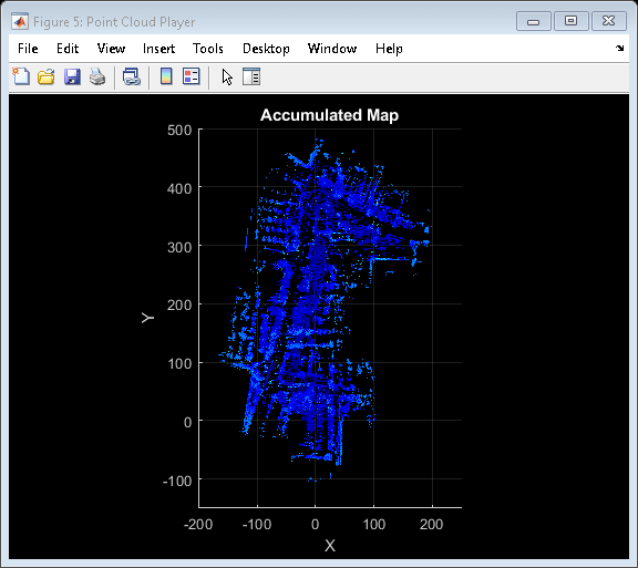
在整个记录数据序列上循环应用预处理和基于特征的注册步骤。结果是一幅车辆所经过的环境地图。

RNG（'默认'）;numFrames =身高(lidarPointClouds);accumTform = rigid3d;pointCloudMap = pointCloud(0, 0, 3);％指定玩家的限制Xlimits = [-200 250];%米Ylimits = [-150 500];Zlimits = [-100 100];%创建一个pc玩家可视化地图mapplayer = pcplayer（xlimits，ylimits，zlimits）;标题（mapplayer.axes，“累积地图”）;mapPlayer.Axes.View =[0,90]; / /视图％循环到整个数据以生成地图为n = 1: skipFrames: numFrames - skipFrames得到第n个点云ptcloud = lidarpointclouds.pointCloud（n）;％段接地并移除自助式车辆ptprocessed = helperprocesspointcloud（ptcloud）;%向下采样点云的运行速度ptDownsampled = pcdownsample (ptProcessed,“gridAverage”, gridStep);%从点云中提取特征[ptFeature, ptValidInds] = extractFPFHFeatures(ptdownsampling, ptValidInds).．.“NumNeighbors”、邻居);ptValidPts = select(ptDownsampled, ptValidInds);如果n==1 moving = ptValidPts;movingFeature = ptFeature;pointCloudMap = ptValidPts;其他的固定=移动;FIRIDEFEATURE =运动;移动= ptvalidpts;移动= ptfeature;匹配特征以找到对应indexPairs = pcmatchfeatures(movingFeature, fixedFeature, moving，.．.固定的,“方法”、方法、“MatchThreshold”，临界点，.．.“RejectRatio”、比例);matchedfixedpts = select（固定，indexPairs（:,2））;matchedmovingpts = select（移动，indexPairs（：，1））;记录移动点云与参考点云tform = eStimationGeometricTransform3d（matchedmovingpts.location，.．.matchedfixedpts.location，“刚性”，“MaxDistance”maxDist,.．.“MaxNumTrials”, maxNumTrails);%计算到原始参考系的累积变换accumTform = rigid3d (tform。T * accumTform.T);对齐并合并移动点云到累积地图pointcloudmap = pcalign（[pointcloudmap，移动]，.．.[Rigid3D，Accultform]，SimplGridStep）;结束％更新映射显示视图(mapPlayer pointCloudMap);结束