2017 is upon us and that means some of you may be going into your annual review or thinking about your career after graduation. Today's guest blogger,Toshi Takeuchiused machine learning on a job-related dataset forpredictive analytics. Let's see what he learned.

Contents

Companies spend money and time recruiting talent and they lose all that investment when people leave. Therefore companies can save money if they can intervene before their employees leave. Perhaps this is a sign of a robust economy, that one of the datasets popular on Kaggle deals with this issue:Human Resources Analytics - Why are our best and most experienced employees leaving prematurely?Note that this dataset is no longer available on Kaggle.

This is an example ofpredictive analyticswhere you try to predict future events based on the historical data using machine learning algorithms. When people talk about predictive analytics, you hear often that the key is to turn insights into action. What does that really mean? Let's also examine this question through exploration of this dataset.

Dataset

The Kaggle page says "our example concerns a big company that wants to understand why some of their best and most experienced employees are leaving prematurely. The company also wishes to predict which valuable employees will leave next."

The fields in the dataset include:

Let's load it into MATLAB. The newdetectImportOptionsmakes it easy to set up import options based on the file content.

opts = detectImportOptions('HR_comma_sep.csv');% set import optionsopts.VariableTypes(9:10) = {'categorical'};% turn text to categoricalcsv = readtable('HR_comma_sep.csv', opts);% import datafprintf(“行数:% d \ n”,height(csv))% show number of rows

Number of rows: 14999

We will then hold out 10% of the dataset for model evaluation (holdout), and use the remaining 90% (train) to explore the data and train predictive models.

rng(1)% for reproducibilityc = cvpartition(csv.left,'HoldOut',0.1);% partition datatrain = csv(training(c),:);% for trainingholdout = csv(test(c),:);% for model evaluation

Big Picture - How Bad Is Turnover at This Company?

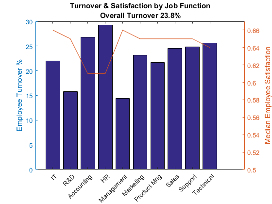
The first thing to understand is how bad a problem this company has. Assuming each row represents an employee, this company employs close to 14999 people over some period and about 24% of them left this company in that same period (not stated). Is this bad? Turnover is usually calculated on an annual basis and we don't know what period this dataset covers. Also the turnover rate differs from industry to industry. That said, this seems pretty high for a company of this size with an internal R&D team.

When you break it down by job function, the turnover seems to be correlated to job satisfaction. For example, HR and accounting have low median satisfaction levels and high turnover ratios where as R&D and Management have higher satisfaction levels and lower turnover ratios.

Please note the use of new functions in R2016b:xticklabelsto set x-axis tick labels andxtickangleto rotate x-axis tick labels.

[g, job] = findgroups(train.sales);% group by salesjob = cellstr(job);% convert to celljob = replace(job,'and','&');% clean upjob = replace(job,'_',' ');% more clean upjob = regexprep(job,'(^| )\s*.','${upper($0)}');% capitalize first letterjob = replace(job,'Hr','HR');% more capitalizefunc = @(x) sum(x)/numel(x);% anonymous functionturnover = splitapply(func, train.left, g);% get group statsfigure% new figureyyaxisleft% left y-axisbar(turnover*100)%营业额百分比xticklabels(job)% label barsxtickangle(45)% rotate labelsylabel('Employee Turnover %')% left y-axis labeltitle({'Turnover & Satisfaction by Job Function';...sprintf('Overall Turnover %.1f%%', sum(train.left)/height(train)*100)}) holdon% overlay another plotsatisfaction = splitapply(@median,...% get group mediantrain.satisfaction_level, g); yyaxisright% right y-axisplot(1:length(job),satisfaction)% plot median lineylabel('Median Employee Satisfaction')% right y-axis labelylim([.5 .67])% scale left y-axisholdoff% stop overlay

Defining Who Are the "Best"

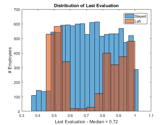
我们被要求分析最好和最费用的原因rienced employees are leaving. How do we identify who are the "best"? For the purpose of this analysis, I will use the performance evaluation score to determine who are high performers. As the following histogram shows, employees with lower scores as well as higher scores tend to leave, and people with average scores are less likely to leave. The median score is 0.72. Let's say anyone with 0.8 or higher scores are high performers.

figure% new figurehistogram(train.last_evaluation(train.left == 0))% histogram of those stayedholdon% overlay another plothistogram(train.last_evaluation(train.left == 1))% histogram of those leftholdoff% stop overlayxlabel(...% x-axis labelsprintf('Last Evaluation - Median = %.2f',median(train.last_evaluation))) ylabel('# Employees')% y-axis labellegend('Stayed','Left')% add legendtitle('Distribution of Last Evaluation')% add title

Defining Who Are the "Most Experienced"

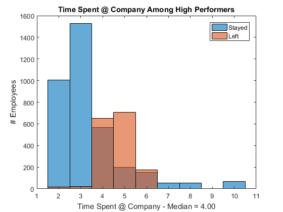
Among high performers, the company is particularly interested in "most experienced" people - let's use Time Spent at Company to measure the experience level. The plot shows that high performers with 4 to 6 years of experience are at higher risk of turnover.

hp = train(train.last_evaluation >= 0.8,:);% subset high performersfigure% new figurehistogram(hp.time_spend_company(hp.left == 0))% histogram of those stayedholdon% overlay another plothistogram(hp.time_spend_company(hp.left == 1))% histogram of those leftholdoff% stop overlayxlabel(...% x-axis labelsprintf('Time Spent @ Company - Median = %.2f',median(hp.time_spend_company))) ylabel('# Employees')% y-axis labellegend('Stayed','Left')% add legendtitle(“@公司表现在高时间”)% add title

Job Satisfaction Among High Risk Group

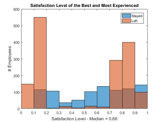
Let's isolate the at-risk group and see how their job satisfaction stacks up. It is interesting to see that not only people with very low satisfaction levels (no surprise) but also the highly satisfied people left the company. It seems like people with a satisfaction level of 0.7 or higher are at an elevated risk.

at_risk = hp(hp.time_spend_company >= 4 &...% subset high performershp.time_spend_company <= 6,:);% with 4-6 years experiencefigure% new figurehistogram(at_risk.satisfaction_level(...% histogram of those stayedat_risk.left == 0)) holdon% overlay another plothistogram(at_risk.satisfaction_level(...% histogram of those leftat_risk.left == 1)) holdoff% stop overlayxlabel(...% x-axis labelsprintf('Satisfaction Level - Median = %.2f',median(at_risk.satisfaction_level))) ylabel('# Employees')% y-axis labellegend('Stayed','Left')% add legendtitle('Satisfaction Level of the Best and Most Experienced')

Was It for Money?

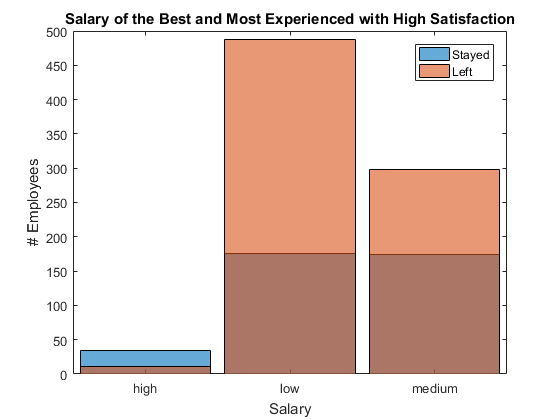
Let's isolate high performing seasoned employees and check their salaries. It is clear that people who get a higher salary are staying while people with medium or low salary leave. No big surprise here, either.

at_risk_sat = at_risk(...% subset at_riskat_risk.satisfaction_level >= .7,:); figure% new figurehistogram(at_risk_sat.salary(at_risk_sat.left == 0))% histogram of those stayedholdon% overlay another plothistogram(at_risk_sat.salary(at_risk_sat.left == 1))% histogram of those leftholdoff% stop overlayxlabel('Salary')% x-axis labelylabel('# Employees')% y-axis labellegend('Stayed','Left')% add legendtitle('Salary of the Best and Most Experienced with High Satisfaction')

Making Insights Actionable with Predictive Analytics

At this point, you may say, "I knew all this stuff already. I didn't get any new insight from this analysis." It's true, but why are you complaining about that?Predictability is a good thing for prediction!

What we have seen so far all happened in the past, which you cannot undo. However, if you can predict the future, you can do something about it. Making data actionable - that's the true value of predictive analytics.

在order to make this insight actionable, we need to quantify the turnover risk as scores so that we can identify at-risk employees for intervention. Since we are trying to classify people into those who are likely to stay vs. leave, what we need to do is build a classification model to predict such binary outcome.

I have used theClassification Learnerapp to run multiple classifiers on our training datatrainto see which one provides the highest prediction accuracy.

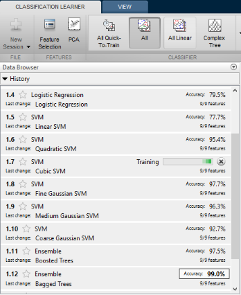
The winner is theBagged Treesclassifier (also known as "Random Forest") with 99.0% accuracy. To evaluate a classifier, we typically use theROC curve plot, which lets you see the trade-off between the true positive rate vs. false positive rate. If you have a high AUC score like 0.99, the classifer is very good at identifying the true class without causing too many false positives.

You can also export the trained predictive model from the Classification Learner. I saved the exported model asbtree.matthat comes with some instructions.

loadbtree% load trained modelhow_to = btree.HowToPredict;% get how to usedisp([how_to(1:80)' ...'])% snow snippet

To make predictions on a new table, T, use: yfit = c.predictFcn(T) replacing ...

Evaluating the Predictive Performance

Let's pick 10 samples from theholdoutdata partition and see how the predictive model scores them. Here are the samples - 5 people who left and 5 who stayed. They are all high performers with 4 or more years of experience.

samples = holdout([111; 484; 652; 715; 737; 1135; 1293; 1443; 1480; 1485],:); samples(:,[1,2,5,8,9,10,7])

ans = satisfaction_level last_evaluation time_spend_company promotion_last_5years sales salary left __________________ _______________ __________________ _____________________ __________ ______ ____ 0.9 0.92 4 0 sales low 1 0.31 0.92 6 0 support medium 0 0.86 0.87 4 0 sales low 0 0.62 0.95 4 0 RandD low 0 0.23 0.96 6 0 marketing medium 0 0.39 0.89 5 0 support low 0 0.09 0.92 4 0 sales medium 1 0.73 0.87 5 0 IT low 1 0.75 0.97 6 0 technical medium 1 0.84 0.83 5 0 accounting low 1

Now let's try the model to predict whether they left the company.

actual = samples.left;% actual outocmepredictors = samples(:,[1:6,8:10]);% predictors only[predicted,score]= btree.predictFcn(predictors);% get predictionc = confusionmat(actual,predicted);% get confusion matrixdisp(array2table(c,...% show the matrix as table'VariableNames',{'Predicted_Stay','Predicted_Leave'},...'RowNames',{'Actual_Stayed','Actual_Left'}));

Predicted_Stay Predicted_Leave ______________ _______________ Actual_Stayed 5 0 Actual_Left 0 5

The model was able to predict the outcome of those 10 samples accurately. In addition, it also returns the probability of each class as score. You can also use the entireholdoutdata to check the model performance, but I will skip that step here.

Using the Model to Take Action

We can use the probability of leaving as the risk score. We can select high performers based on the last evaluation and time spent at the company, and then score their risk level and intervene in high risk cases. In this example, the sales employee with the 0.92 evaluation score is 100% at risk of leaving. Since this employee has not been promoted in the last 5 years, perhaps it is time to do so.

samples.risk = score(:,2);%的概率离开[~,ranking] = sort(samples.risk,'descend');% sort by risk scoresamples = samples(ranking,:);% sort table by rankingsamples(samples.risk > .7,[1,2,5,8,9,10,11])% intervention targets

ans = satisfaction_level last_evaluation time_spend_company promotion_last_5years sales salary risk __________________ _______________ __________________ _____________________ __________ ______ _______ 0.09 0.92 4 0 sales medium 1 0.73 0.87 5 0 IT low 1 0.84 0.83 5 0 accounting low 0.9984 0.75 0.97 6 0 technical medium 0.96154 0.9 0.92 4 0 sales low 0.70144

Explaining the Model

Machine learning algorithms used in predictive analytics are often a black-box solution, so HR managers may need to provide an easy-to-understand explanation about how it works in order to get the buy-in from their superiors. We can use the predictor importance score to show which attributes are used to compute the prediction.

在this example, the model is using the mixture of attributes at different weights to compute it, with emphasis on the satisfaction level, followed by the number of projects and time spent at the company. We also see that people who got a promotion in the last 5 years are less likely to leave. Those attributes are very obvious and therefore we feel more confident about the prediction with this model.

imp = oobPermutedPredictorImportance(...% get predictor importancebtree.ClassificationEnsemble); vals = btree.ClassificationEnsemble.PredictorNames;% predictor namesfigure% new figurebar(imp);% plot importnacetitle('Out-of-Bag Permuted Predictor Importance Estimates'); ylabel('Estimates');% y-axis labelxlabel('Predictors');% x-axis labelxticklabels(vals)% label barsxtickangle(45)% rotate labelsax = gca;% get current axesax.TickLabelInterpreter ='none';% turn off latex

Operationalizing Action

The predictor importance score also give us a hint about when we should intervene. Given that satisfaction level, last evaluation, and time spent at the company are all important predictors, it is probably a good idea to update the predictive scores at the time of each annual evaluation and then decide who may need intervention.

It is feasible to implement a system to schedule such analysis when a performance review is conducted and automatically generate a report of high risk employees using the model derived from MATLAB. Here isa simple live demoof such a system running the following code using MATLAB Production Server. It uses the trained predictive model we just generated.

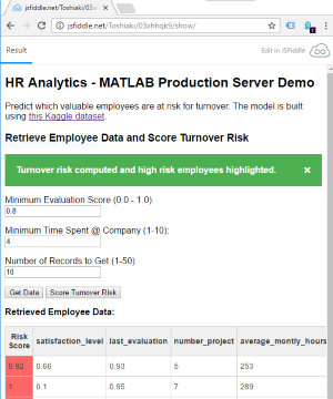
The example code just loads the data from MAT-file, but you would instead access data from anSQL databasein a real world use scenario. Please also note the use of a new functionjsonencodeintroduced in R2016b that converts structure arrays into JSON formatted text. Naturally, we also havejsondecodethat converts JSON formatted text into appropriate MATLAB data types.

dbtypescoreRisk.m

1 function risk = scoreRisk(employee_ids) 2 %SCORERISK scores the turnover risk of selected employees 3 4 load data % load holdout data 5 load btree % load trained model 6 X_sub = X(employee_ids,:); % select employees 7 [predicted,score]= btree.predictFcn(X_sub); % get prediction 8 risk = struct('Ypred',predicted,'score',score(:,2));% create struct 9 risk = jsonencode(risk); % JSON encode it 10 11 end

Depending on your needs, you can build it in a couple of ways:

Often, you would need to retrain the predictive model as human behavior changes over time. If you use code generated from MATLAB, it is very easy to retrain using the new dataset and redeploy the new model for production use, as compared to cases where you reimplement the model in some other languages.

Summary

在the beginning of this analysis, we explored the dataset which represents the past. You cannot undo the past, but you can do something about the future if you can find quantifiable patterns in the data for prediction.

People often think the novelty of insights is important. What really matters is what action you can take on them, whether novel or well-known. If you do nothing, no fancy analytics will deliver any value. Harvard Business Review recently publushed an article为什么哟u’re Not Getting Value from Your Data Sciencebut failed to mention this issue.

在my opionion,analysis paralysisis one of the biggest reason companies are not getting the value because they are failing to take action and are stuck at the data analysis phase of the data science process.

Has this example helped you understand how you can use predictive analytics to solve practical problems? Can you think of way to apply this in your area of work? Let us know what you thinkhere.

Get the MATLAB code

Published with MATLAB® R2016b