Assess Stationarity of Time Series Using Econometric Modeler

These examples show how to conduct statistical hypothesis tests for assessing whether a time series is a unit root process by using the Econometric Modeler app. The test you use depends on your assumptions about the nature of the nonstationarity of an underlying model.

Test Assuming Unit Root Null Model

This example uses the Augmented Dickey-Fuller and Phillips-Perron tests to assess whether a time series is a unit root process. The null hypothesis for both tests is that the time series is a unit root process. The data set, stored inData_USEconModel.mat, contains the US gross domestic product (GDP) measured quarterly, among other series.

At the command line, load theData_USEconModel.matdata set.

loadData_USEconModel

At the command line, open theEconometric Modeler应用程序。

econometricModeler

Alternatively, open the app from the apps gallery (seeEconometric Modeler).

ImportDataTableinto the app:

On theEconometric Modelertab, in theImportsection, click.
In theImport Datadialog box, in theImport?column, select the check box for theDataTablevariable.
ClickImport.

The variables, amongGDP, appear in theTime Seriespane, and a time series plot of all the series appears in theTime Series Plot(COE)figure window.

In theTime Series窗格中,double-clickGDP. A time series plot ofGDPappears in theTime Series Plot(GDP)figure window.

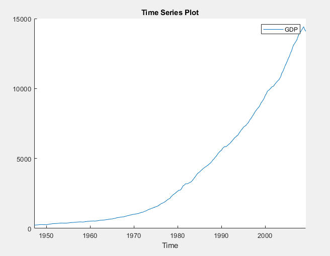
The series appears to grow without bound.

Apply the log transformation toGDP. On theEconometric Modelertab, in theTransformssection, clickLog.

In theTime Seriespane, a variable representing the logged GDP (GDPLog) appears. A time series plot of the logged GDP appears in theTime Series Plot(GDPLog)figure window.

The logged GDP series appears to have a time trend or drift term.

Using the Augmented Dickey-Fuller test, test the null hypothesis that the logged GDP series has a unit root against a trend stationary AR(1) model alternative. Conduct a separate test for an AR(1) model with drift alternative. For the null hypothesis of both tests, include the restriction that the trend and drift terms, respectively, are zero by conductingFtests.

WithGDPLogselected in theTime Seriespane, on theEconometric Modelertab, in theTestssection, clickNew Test>Augmented Dickey-Fuller Test.
On theADFtab, in theParameterssection:
1. SetNumber of Lagsto1.
2. SelectModel>Trend Stationary.
3. SelectTest Statistic>F statistic.
In theTestssection, clickRun Test.
Repeat steps 2 and 3, but selectModel>Autoregressive with Driftinstead.

The test results appear in theResultstable of theADF(GDPLog)document.

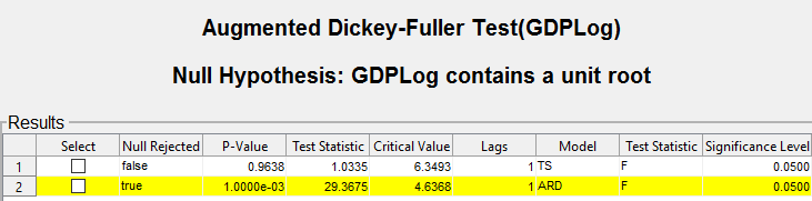
For the test supposing a trend stationary AR(1) model alternative, the null hypothesis is not rejected. For the test assuming an AR(1) model with drift, the null hypothesis is rejected.

Apply the Phillips-Perron test using the same assumptions as in the Augmented Dickey-Fuller tests, except the trend and drift terms in the null model cannot be zero.

WithGDPLogselected in theTime Seriespane, click theEconometric Modelertab. Then, in theTestssection, clickNew Test>Phillips-Perron Test.
On thePPtab, in theParameterssection:
1. SetNumber of Lagsto1.
2. SelectModel>Trend Stationary.
In theTestssection, clickRun Test.
Repeat steps 2 and 3, but selectModel>Autoregressive with Driftinstead.

The test results appear in theResultstable of thePP(GDPLog)document.

The null is not rejected for both tests. These results suggest that the logged GDP possibly has a unit root.

The difference in the null models can account for the differences between the Augmented Dickey-Fuller and Phillips-Perron test results.

Test Assuming Stationary Null Model

This example uses the Kwiatkowski, Phillips, Schmidt, and Shin (KPSS) test to assess whether a time series is a unit root process. The null hypothesis is that the time series is stationary. The data set, stored inData_NelsonPlosser.mat, contains annual nominal wages, among other US macroeconomic series.

At the command line, load theData_NelsonPlosser.matdata set.

loadData_NelsonPlosser

Convert the tableDataTableto a timetable (for details, seePrepare Time Series Data for Econometric Modeler App).

dates = datetime(dates,12,31,'Format','yyyy');% Convert dates to datetimesDataTable.Properties.RowNames = {};% Clear row namesDataTable = table2timetable(DataTable,'RowTimes',dates);% Convert table to timetable

At the command line, open theEconometric Modeler应用程序。

econometricModeler

Alternatively, open the app from the apps gallery (seeEconometric Modeler).

ImportDataTableinto the app:

On theEconometric Modelertab, in theImportsection, click.
In theImport Datadialog box, in theImport?column, select the check box for theDataTablevariable.
ClickImport.

The variables, including the nominal wagesWN, appear in theTime Seriespane, and a time series plot of all the series appears in theTime Series Plot(BY)figure window.

In theTime Series窗格中,double-clickWN. A time series plot ofWNappears in theTime Series Plot(WN)figure window.

The series appears to grow without bound, and wage measurements are missing before 1900. To zoom into values occurring after 1900, pause on the plot, click盒子里,将时间序列刺激uced by dragging the cross hair.

Apply the log transformation toWN. On theEconometric Modelertab, in theTransformssection, clickLog.

In theTime Seriespane, a variable representing the logged wages (WNLog) appears. The logged series appears in theTime Series Plot(WNLog)figure window.

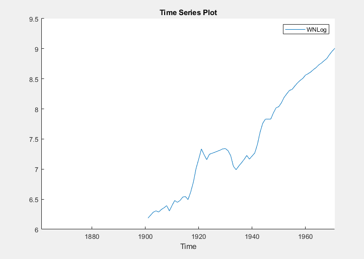
The logged wages appear to have a linear trend.

Using the KPSS test, test the null hypothesis that the logged wages are trend stationary against the unit root alternative. As suggested in[1], conduct three separate tests by specifying 7, 9, and 11 lags in the autoregressive model.

WithWNLogselected in theTime Seriespane, on theEconometric Modelertab, in theTestssection, clickNew Test>KPSS Test.
On theKPSStab, in theParameterssection, setNumber of Lagsto7.
In theTestssection, clickRun Test.
Repeat steps 2 and 3, but setNumber of Lagsto9instead.
Repeat steps 2 and 3, but setNumber of Lagsto11instead.

The test results appear in theResultstable of theKPSS(WNLog)document.

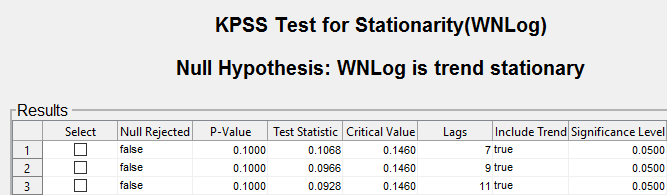
All tests fail to reject the null hypothesis that the logged wages are trend stationary.

Test Assuming Random Walk Null Model

This example uses the variance ratio test to assess the null hypothesis that a time series is a random walk. The data set, stored inCAPMuniverse.mat, contains market data for daily returns of stocks and cash (money market) from the period January 1, 2000 to November 7, 2005.

At the command line, load theCAPMuniverse.matdata set.

loadCAPMuniverse

The series are in the timetableAssetsTimeTable. The first column of data (AAPL) is the daily return of a technology stock. The last column is the daily return for cash (the daily money market rate,CASH).

Accumulate the daily technology stock and cash returns.

AssetsTimeTable.AAPLcumsum = cumsum(AssetsTimeTable.AAPL); AssetsTimeTable.CASHcumsum = cumsum(AssetsTimeTable.CASH);

At the command line, open theEconometric Modeler应用程序。

econometricModeler

Alternatively, open the app from the apps gallery (seeEconometric Modeler).

ImportAssetsTimeTableinto the app:

On theEconometric Modelertab, in theImportsection, click.
In theImport Datadialog box, in theImport?column, select the check box for theAssetsTimeTablevariable.
ClickImport.

The variables, including stock and cash prices (AAPLcumsumandCASHcumsum), appear in theTime Seriespane, and a time series plot of all the series appears in theTime Series Plot(AAPL)figure window.

In theTime Series窗格中,double-clickAAPLcumsum. A time series plot ofAAPLcumsumappears in theTime Series Plot(AAPLcumsum)figure window.

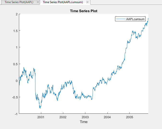
The accumulated returns of the stock appear to wander at first, with high variability, and then grow without bound after 2004.

Using the variance ratio test, test the null hypothesis that the series of accumulated stock returns is a random walk. First, test without assuming IID innovations for the alternative model, then test assuming IID innovations.

WithAAPLcumsumselected in theTime Seriespane, on theEconometric Modelertab, in theTestssection, clickNew Test>Variance Ratio Test.
On theVRatiotab, in theTestssection, clickRun Test.
On theVRatiotab, in theParameterssection, select theIID Innovationscheck box.
In theTestssection, clickRun Test.

The test results appear in theResultstable of theVRatio(AAPLcumsum)document.

Without assuming IID innovations for the alternative model, the test fails to reject the random walk null model. However, assuming IID innovations, the test rejects the null hypothesis. This result might be due to heteroscedasticity in the series, that is, the series might be a heteroscedastic random walk.

In theTime Series窗格中,double-clickCASHcumsum. A time series plot ofCASHcumsumappears in theTime Series Plot(CASHcumsum)figure window.

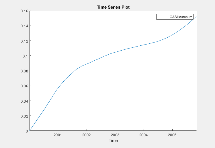
The series of accumulated cash returns exhibits low variability and appears to have long-term trends.

Test the null hypothesis that the series of accumulated cash returns is a random walk:

WithCASHcumsumselected in theTime Seriespane, on theEconometric Modelertab, in theTestssection, clickNew Test>Variance Ratio Test.
On theVRatiotab, in theParameterssection, clear theIID Innovationsbox.
In theTestssection, clickRun Test.

The test results appear in theResultstab of theVRatio(CASHcumsum)document.

The test rejects the null hypothesis that the series of accumulated cash returns is a random walk.

References

[1]Kwiatkowski, D., P. C. B. Phillips, P. Schmidt, and Y. Shin. “Testing the Null Hypothesis of Stationarity against the Alternative of a Unit Root.”Journal of Econometrics. Vol. 54, 1992, pp. 159–178.