pdf

Probability density function

collapse all in page

Syntax

y = pdf('name',x,A)

y = pdf('name',x,A,B)

y = pdf('name',x,A,B,C)

y = pdf('name',x,A,B,C,D)

y = pdf(pd,x)

Description

example

y = pdf('name',x,A) returns the probability density function (pdf) for the one-parameter distribution family specified by 'name' and the distribution parameter A, evaluated at the values in x.

example

y = pdf('name',x,A,B) returns the pdf for the two-parameter distribution family specified by 'name' and the distribution parameters A and B, evaluated at the values in x.

y = pdf('name',x,A,B,C) returns the pdf for the three-parameter distribution family specified by 'name' and the distribution parameters A, B, and C, evaluated at the values in x.

y = pdf('name',x,A,B,C,D) returns the pdf for the four-parameter distribution family specified by 'name' and the distribution parameters A, B, C, and D, evaluated at the values in x.

example

y = pdf(pd,x) returns the pdf of the probability distribution object pd, evaluated at the values in x.

Examples

collapse all

Compute the Normal Distribution pdf

Open Live Script

Create a standard normal distribution object with the mean $μ$ equal to 0 and the standard deviation $σ$ equal to 1.

mu = 0;
sigma = 1;
pd = makedist('Normal','mu',mu,'sigma',sigma);

Define the input vector x to contain the values at which to calculate the pdf.

x = [-2 -1 0 1 2];

Compute the pdf values for the standard normal distribution at the values in x.

y = pdf(pd,x)

y = 1×5

    0.0540    0.2420    0.3989    0.2420    0.0540

Each value in y corresponds to a value in the input vector x. For example, at the value x equal to 1, the corresponding pdf value y is equal to 0.2420.

Alternatively, you can compute the same pdf values without creating a probability distribution object. Use the pdf function, and specify a standard normal distribution using the same parameter values for $μ$ and $σ$ .

y2 = pdf('Normal',x,mu,sigma)

y2 = 1×5

    0.0540    0.2420    0.3989    0.2420    0.0540

The pdf values are the same as those computed using the probability distribution object.

Compute the Poisson Distribution pdf

Open Live Script

Create a Poisson distribution object with the rate parameter, $λ$ , equal to 2.

lambda = 2;
pd = makedist('Poisson','lambda',lambda);

Define the input vector x to contain the values at which to calculate the pdf.

x = [0 1 2 3 4];

Compute the pdf values for the Poisson distribution at the values in x.

y = pdf(pd,x)

y = 1×5

    0.1353    0.2707    0.2707    0.1804    0.0902

Each value in y corresponds to a value in the input vector x. For example, at the value x equal to 3, the corresponding pdf value in y is equal to 0.1804.

Alternatively, you can compute the same pdf values without creating a probability distribution object. Use the pdf function, and specify a Poisson distribution using the same value for the rate parameter, $λ$ .

y2 = pdf('Poisson',x,lambda)

y2 = 1×5

    0.1353    0.2707    0.2707    0.1804    0.0902

The pdf values are the same as those computed using the probability distribution object.

Plot the pdf of a Standard Normal Distribution

Open Live Script

Create a standard normal distribution object.

pd = makedist('Normal')

pd = 
  NormalDistribution

  Normal distribution
       mu = 0
    sigma = 1

Specify the x values and compute the pdf.

x = -3:.1:3;
pdf_normal = pdf(pd,x);

Plot the pdf.

plot(x,pdf_normal,'LineWidth',2)

Plot the pdf of a Weibull Distribution

Open Live Script

Create a Weibull probability distribution object.

pd = makedist('Weibull','a',5,'b',2)

pd = 
  WeibullDistribution

  Weibull distribution
    A = 5
    B = 2

Specify the x values and compute the pdf.

x = 0:.1:15;
y = pdf(pd,x);

Plot the pdf.

plot(x,y,'LineWidth',2)

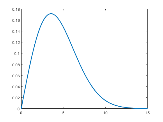
Input Arguments

collapse all

`'name'` — Probability distribution name
character vector or string scalar of probability distribution name

Probability distribution name, specified as one of the probability distribution names in this table.

`'name'`	Distribution	Input Parameter `A`	Input Parameter `B`	Input Parameter `C`	Input Parameter `D`
`'Beta'`	Beta Distribution	a first shape parameter	b second shape parameter	—	—
`'Binomial'`	Binomial Distribution	n number of trials	p probability of success for each trial	—	—
`'BirnbaumSaunders'`	Birnbaum-Saunders Distribution	β scale parameter	γ shape parameter	—	—
`'Burr'`	Burr Type XII Distribution	α scale parameter	c first shape parameter	k second shape parameter	—
`'Chisquare'`	Chi-Square Distribution	ν degrees of freedom	—	—	—
`'Exponential'`	Exponential Distribution	μ mean	—	—	—
`'Extreme Value'`	Extreme Value Distribution	μ location parameter	σ scale parameter	—	—
`'F'`	F Distribution	ν₁ numerator degrees of freedom	ν₂ denominator degrees of freedom	—	—
`'Gamma'`	Gamma Distribution	a shape parameter	b scale parameter	—	—
`'Generalized Extreme Value'`	Generalized Extreme Value Distribution	k shape parameter	σ scale parameter	μ location parameter	—
`'Generalized Pareto'`	Generalized Pareto Distribution	k tail index (shape) parameter	σ scale parameter	μ threshold (location) parameter	—
`'Geometric'`	Geometric Distribution	p probability parameter	—	—	—
`'HalfNormal'`	Half-Normal Distribution	μ location parameter	σ scale parameter	—	—
`'Hypergeometric'`	Hypergeometric Distribution	m size of the population	k number of items with the desired characteristic in the population	n number of samples drawn	—
`'InverseGaussian'`	Inverse Gaussian Distribution	μ scale parameter	λ shape parameter	—	—
`'Logistic'`	Logistic Distribution	μ mean	σ scale parameter	—	—
`'LogLogistic'`	Loglogistic Distribution	μ mean of logarithmic values	σ scale parameter of logarithmic values	—	—
`'Lognormal'`	Lognormal Distribution	μ mean of logarithmic values	σ standard deviation of logarithmic values	—	—
`'Nakagami'`	Nakagami Distribution	μ shape parameter	ω scale parameter	—	—
`'Negative Binomial'`	Negative Binomial Distribution	r number of successes	p probability of success in a single trial	—	—
`'Noncentral F'`	Noncentral F Distribution	ν₁ numerator degrees of freedom	ν₂ denominator degrees of freedom	δ noncentrality parameter	—
`'Noncentral t'`	Noncentral t Distribution	ν degrees of freedom	δ noncentrality parameter	—	—
`'Noncentral Chi-square'`	Noncentral Chi-Square Distribution	ν degrees of freedom	δ noncentrality parameter	—	—
`'Normal'`	Normal Distribution	μ mean	σ standard deviation	—	—
`'Poisson'`	Poisson Distribution	λ mean	—	—	—
`'Rayleigh'`	Rayleigh Distribution	b scale parameter	—	—	—
`'Rician'`	Rician Distribution	s noncentrality parameter	σ scale parameter	—	—
`'Stable'`	Stable Distribution	α first shape parameter	β second shape parameter	γ scale parameter	δ location parameter
`'T'`	Student's t Distribution	ν degrees of freedom	—	—	—
`'tLocationScale'`	t Location-Scale Distribution	μ location parameter	σ scale parameter	ν shape parameter	—
`'Uniform'`	Uniform Distribution (Continuous)	a lower endpoint (minimum)	b upper endpoint (maximum)	—	—
`'Discrete Uniform'`	Uniform Distribution (Discrete)	n maximum observable value	—	—	—
`'Weibull'`	Weibull Distribution	a scale parameter	b shape parameter	—	—

Example: 'Normal'

`x` — Values at which to evaluate pdf
scalar value | array of scalar values

Values at which to evaluate the pdf, specified as a scalar value or an array of scalar values.

If one or more of the input arguments x, A, B, C, and D are arrays, then the array sizes must be the same. In this case, pdf expands each scalar input into a constant array of the same size as the array inputs. See 'name' for the definitions of A, B, C, and D for each distribution.

Example: [-1,0,3,4]